The prediction of long non-coding RNA (lncRNA) subcellular localization is essential to the understanding of its function and involvement in cellular regulation. Traditional biological experimental methods are costly and time-consuming, making computational methods the preferred approach for predicting lncRNA subcellular localization (LSL). However, existing computational methods have limitations due to the structural characteristics of lncRNAs and the uneven distribution of data across subcellular compartments. We propose a discrete wavelet transform (DWT)-based model for predicting LSL, called DlncRNALoc. We construct a physicochemical property matrix of a 2-tuple bases based on lncRNA sequences, and we introduce a DWT lncRNA feature extraction method. We use the Synthetic Minority Over-sampling Technique (SMOTE) for oversampling and the local fisher discriminant analysis (LFDA) algorithm to optimize feature information. The optimized feature vectors are fed into support vector machine (SVM) to construct a predictive model. DlncRNALoc has been applied for a five-fold cross-validation on the three sets of benchmark datasets. Extensive experiments have demonstrated the superiority and effectiveness of the DlncRNALoc model in predicting LSL.
Citation: Xiangzheng Fu, Yifan Chen, Sha Tian. DlncRNALoc: A discrete wavelet transform-based model for predicting lncRNA subcellular localization[J]. Mathematical Biosciences and Engineering, 2023, 20(12): 20648-20667. doi: 10.3934/mbe.2023913
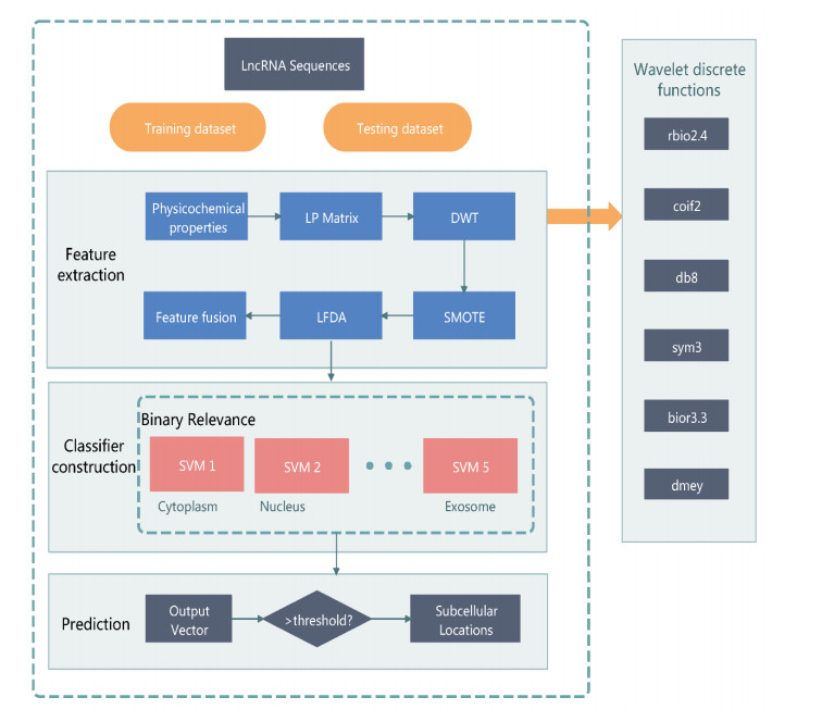
The prediction of long non-coding RNA (lncRNA) subcellular localization is essential to the understanding of its function and involvement in cellular regulation. Traditional biological experimental methods are costly and time-consuming, making computational methods the preferred approach for predicting lncRNA subcellular localization (LSL). However, existing computational methods have limitations due to the structural characteristics of lncRNAs and the uneven distribution of data across subcellular compartments. We propose a discrete wavelet transform (DWT)-based model for predicting LSL, called DlncRNALoc. We construct a physicochemical property matrix of a 2-tuple bases based on lncRNA sequences, and we introduce a DWT lncRNA feature extraction method. We use the Synthetic Minority Over-sampling Technique (SMOTE) for oversampling and the local fisher discriminant analysis (LFDA) algorithm to optimize feature information. The optimized feature vectors are fed into support vector machine (SVM) to construct a predictive model. DlncRNALoc has been applied for a five-fold cross-validation on the three sets of benchmark datasets. Extensive experiments have demonstrated the superiority and effectiveness of the DlncRNALoc model in predicting LSL.

| [1] |
Y. Wu, S. Ma, Impact of COVID-19 on energy prices and main macroeconomic indicators—evidence from China's energy market, Green Finance, 3 (2021), 383–402. https://doi.org/10.3934/GF.2021019 doi: 10.3934/GF.2021019

|
| [2] |
E. Assifuah-Nunoo, P. O. Junior, A. M. Adam, B. Ahmed, Assessing the safe haven properties of oil in African stock markets amid the COVID-19 pandemic: a quantile regression analysis, Quant. Finance Econ., 6 (2022), 244–269. https://doi.org/10.3934/QFE.2022011 doi: 10.3934/QFE.2022011
|
| [3] |
L. Katusiime, Time-Frequency connectedness between developing countries in the COVID-19 pandemic: The case of East Africa, Quant. Finance Econ., 6 (2022), 722–748. https://doi.org/10.3934/QFE.2022032 doi: 10.3934/QFE.2022032
|
| [4] |
Z. Li, B. Mo, H. Nie, Time and frequency dynamic connectedness between cryptocurrencies and financial assets in China, Int. Rev. Econ. Finance, 86 (2023), 46–57. https://doi.org/10.1016/j.iref.2023.01.015 doi: 10.1016/j.iref.2023.01.015
|
| [5] |
A. Narvekar, D. Guha, Bankruptcy prediction using machine learning and an application to the case of the COVID-19 recession, Data Sci. Finance Econ., 1 (2021), 180–195. https://doi.org/10.3934/DSFE.2021010 doi: 10.3934/DSFE.2021010
|
| [6] |
Q. Yang, F. Lin, Y. Wang, M. Zeng, M. Luo, Long noncoding RNAs as emerging regulators of COVID-19, Front. Immunol., 12 (2021), 700184. https://doi.org/10.3389/fimmu.2021.700184 doi: 10.3389/fimmu.2021.700184
|
| [7] |
R. Wu, Y. Su, H. Wu, Y. Dai, M. Zhao, Q. Lu, Characters, functions and clinical perspectives of long non-coding RNAs, Mol. Genet. Genomics, 291 (2016), 1013–1033. https://doi.org/10.1007/s00438-016-1179-y doi: 10.1007/s00438-016-1179-y
|
| [8] |
Z. Cao, X. Pan, Y. Yang, Y. Huang, H. Shen, The lncLocator: a subcellular localization predictor for long non-coding RNAs based on a stacked ensemble classifier, Bioinformatics, 34 (2018), 2185–2194. https://doi.org/10.1093/bioinformatics/bty085 doi: 10.1093/bioinformatics/bty085
|
| [9] |
K. Chou, H. Shen, Cell-PLoc: a package of Web servers for predicting subcellular localization of proteins in various organisms, Nat. Protoc., 3 (2008), 153–162. https://doi.org/10.1038/nprot.2007.494 doi: 10.1038/nprot.2007.494
|
| [10] |
J. Brennecke, A. Stark, R. B. Russell, S. M Cohen, Principles of MicroRNA–target recognition, PLoS Biol., 3 (2005). https://doi.org/10.1371/journal.pbio.0030085 doi: 10.1371/journal.pbio.0030085
|
| [11] |
J. Wei, L. Zhuo, S. Pan, X. Lian, X. Yao, X. Fu, HeadTailTransfer: An efficient sampling method to improve the performance of graph neural network method in predicting sparse ncRNA-protein interactions, Comput. Biol. Med., 157 (2023), 106783. https://doi.org/10.1016/j.compbiomed.2023.106783 doi: 10.1016/j.compbiomed.2023.106783
|
| [12] |
L. Peng, J. Tan, W. Xiong, L. Zhang, Z. Wang, R. Yuan, et al., Deciphering ligand–receptor-mediated intercellular communication based on ensemble deep learning and the joint scoring strategy from single-cell transcriptomic data, Comput. Biol. Med., 163 (2023), 107137. https://doi.org/10.1016/j.compbiomed.2023.107137 doi: 10.1016/j.compbiomed.2023.107137
|
| [13] |
L. Peng, R. Yuan, C. Han, G. Han; J. Tan, Z. Wang, et al., CellEnBoost: A boosting-based ligand-receptor interaction identification model for cell-to-cell communication inference, IEEE Trans. Nanobiosci., 22 (2023), 705–715. https://doi.org/10.1109/TNB.2023.3278685 doi: 10.1109/TNB.2023.3278685
|
| [14] |
L. Cai, X. Ren, X. Fu, L. Peng, M. Gao, X. Zeng, iEnhancer-XG: interpretable sequence-based enhancers and their strength predictor, Bioinformatics, 37 (2020), 1060–1067. https://doi.org/10.1093/bioinformatics/btaa914 doi: 10.1093/bioinformatics/btaa914
|
| [15] |
L. Cai, X. Ren, X. Fu, M. Gao, P. Wang, J. Xu, et al., iEnhancer-CLA: Self-attention-based interpretable model for enhancers and their strength prediction, bioRxiv, 2021. https://doi.org/10.1101/2021.11.23.469658 doi: 10.1101/2021.11.23.469658
|
| [16] |
L. Zhuo, B. Song, Y. Liu, Z. Li, X. Fu, Predicting ncRNA-protein interactions based on dual graph convolutional network and pairwise learning, Briefings Bioinf., 23 (2022). https://doi.org/10.1093/bib/bbac339 doi: 10.1093/bib/bbac339
|
| [17] |
Z. Zhou, Z. Du, J. Wei, L. Zhuo, S. Pan, X. Fu, et al., MHAM-NPI: Predicting ncRNA-protein interactions based on multi-head attention mechanism, Comput. Biol. Med., 163 (2023), 107143. https://doi.org/10.1016/j.compbiomed.2023.107143 doi: 10.1016/j.compbiomed.2023.107143
|
| [18] |
W. Liu, T. Tang, X. Lu, X. Fu, Y. Yang, L. Peng, MPCLCDA: predicting circRNA-disease associations by using automatically selected meta-path and contrastive learning, Briefings Bioinf., 24 (2023). https://doi.org/10.1093/bib/bbad227 doi: 10.1093/bib/bbad227
|
| [19] |
L. Peng, C. Yang, Y. Chen, W. Liu, Predicting CircRNA-disease associations via feature convolution learning with heterogeneous graph attention network, IEEE J. Biomed. Health. Inf., 27 (2023), 3072–3082. https://doi.org/10.1109/JBHI.2023.3260863 doi: 10.1109/JBHI.2023.3260863
|
| [20] |
Z. Li, Y. Zhang, Y. Bai, X. Xie, L. Zeng, IMC-MDA: Prediction of miRNA-disease association based on induction matrix completion, Math. Biosci. Eng., 20 (2023), 10659–10674. https://doi.org/10.3934/mbe.2023471 doi: 10.3934/mbe.2023471
|
| [21] |
J. Wei, L. Zhuo, Z. Zhou, X. Lian, X. Fu, X. Yao, GCFMCL: predicting miRNA-drug sensitivity using graph collaborative filtering and multi-view contrastive learning, Briefings Bioinf., 24 (2023). https://doi.org/10.1093/bib/bbad247 doi: 10.1093/bib/bbad247
|
| [22] |
X. Fu, W. Zhu, L. Cai, B. Liao, L. Peng, Y. Chen, et al., Improved Pre-miRNAs Identification Through Mutual Information of Pre-miRNA Sequences and Structures, Front. Genet., 10 (2019). https://doi.org/10.3389/fgene.2019.00119 doi: 10.3389/fgene.2019.00119
|
| [23] |
Q. Qu, X. Che, B. Ning, X. Zhang, H. Ni, L. Zeng, et al., Prediction of miRNA-disease associations by neural network-based deep matrix factorization, Methods, 212 (2023), 1–9. https://doi.org/10.1016/j.ymeth.2023.02.003 doi: 10.1016/j.ymeth.2023.02.003
|
| [24] |
W. F. Lawless, Autonomous human-machine teams: Reality constrains logic, but hides the complexity of data dependency, Data Sci. Finance Econ., 2 (2022), 464–499. https://doi.org/10.3934/DSFE.2022023 doi: 10.3934/DSFE.2022023
|
| [25] |
L. Peng, F. Wang, Z. Wang, J. Tan, L. Huang, X. Tian, et al., Cell–cell communication inference and analysis in the tumour microenvironments from single-cell transcriptomics: data resources and computational strategies, Briefings Bioinf., 23 (2022), bbac234. https://doi.org/10.1093/bib/bbac234 doi: 10.1093/bib/bbac234
|
| [26] |
Z. Li, L. Ang, W. Shi, N. Xin, M. Chen, H. Tang, Informative SNP selection based on a fuzzy clustering and improved binary particle swarm optimization algorithm, Comput. Math. Methods Med., 2022 (2022). https://doi.org/10.1155/2022/3837579 doi: 10.1155/2022/3837579
|
| [27] |
P. Zweifel, Expanding insurability through exploiting linear partial information, Data Sci. Finance Econ., 2 (2022), 1–16. https://doi.org/10.3934/DSFE.2022001 doi: 10.3934/DSFE.2022001
|
| [28] |
A. Pierleoni, P. L. Martelli, R. Casadio, MemLoci: predicting subcellular localization of membrane proteins in eukaryotes, Bioinformatics, 27 (2011), 1224–1230. https://doi.org/10.1093/bioinformatics/btr108 doi: 10.1093/bioinformatics/btr108
|
| [29] |
H. Shen, K. Chou, Hum-mPLoc: An ensemble classifier for large-scale human protein subcellular location prediction by incorporating samples with multiple sites, Biochem. Biophys. Res. Commun., 355 (2007), 1006–1011. https://doi.org/10.1016/j.bbrc.2007.02.071 doi: 10.1016/j.bbrc.2007.02.071
|
| [30] |
L. Cai, L. Wang, X. Fu, C. Xia, X. Zeng, Q. Zou, ITP-Pred: an interpretable method for predicting, therapeutic peptides with fused features low-dimension representation, Briefings Bioinf., 22 (2020). https://doi.org/10.1093/bib/bbaa367 doi: 10.1093/bib/bbaa367
|
| [31] |
X. Fu, W. Zhu, B. Liao, L. Cai, L. Peng, J. Yang, Improved DNA-Binding protein identification by incorporating evolutionary information into the Chou's PseAAC, IEEE Access, 6 (2018), 66545–66556. https://doi.org/10.1109/ACCESS.2018.2876656 doi: 10.1109/ACCESS.2018.2876656
|
| [32] |
X. Fu, L. Cai, X. Zeng, Q. Zou, StackCPPred: a stacking and pairwise energy content-based prediction of cell-penetrating peptides and their uptake efficiency, Bioinformatics, 36 (2020). https://doi.org/10.1093/bioinformatics/btaa131 doi: 10.1093/bioinformatics/btaa131
|
| [33] |
L. Cai, L. Wang, X. Fu, X. Zeng, Active Semisupervised model for improving the identification of anticancer peptides, ACS Omega, 6 (2021), 23998–24008. https://doi.org/10.1021/acsomega.1c03132 doi: 10.1021/acsomega.1c03132
|
| [34] | Y. Wang, Y. Zhai, Y. Ding, Q. Zou, SBSM-Pro: Support bio-sequence machine for proteins, 2023, preprint, arXiv: 230810275. https://doi.org/10.48550/arXiv.2308.10275 |
| [35] |
R. Wang, Z. Zhou, X. Wu, X. Jiang, L. Zhuo, M. Liu, et al., An effective plant small secretory peptide recognition model based on feature correction strategy, J. Chem. Inf. Model., 2023 (2023). https://doi.org/10.1021/acs.jcim.3c00868 doi: 10.1021/acs.jcim.3c00868
|
| [36] |
H. Shen, K. Chou, PseAAC: a flexible web server for generating various kinds of protein pseudo amino acid composition, Anal. Biochem., 373 (2008), 386–388. https://doi.org/10.1016/j.ab.2007.10.012 doi: 10.1016/j.ab.2007.10.012
|
| [37] |
L. Chen, G. G. Carmichael, Decoding the function of nuclear long non-coding RNAs, Curr. Opin. Cell Biol., 22 (2010), 357–364. https://doi.org/10.1016/j.ceb.2010.03.003 doi: 10.1016/j.ceb.2010.03.003
|
| [38] |
M. N. Cabili, M. C. Dunagin, P. D. McClanahan, A. Biaesch, O. Padovan-Merhar, A. Regev, et al., Localization and abundance analysis of human lncRNAs at single-cell and single-molecule resolution, Genome Biol., 16 (2015), 1–16. https://doi.org/10.1186/s13059-015-0586-4 doi: 10.1186/s13059-015-0586-4
|
| [39] |
T. Zhang, P. Tan, L. Wang, N. Jin, Y. Li, L. Zhang, et al., RNALocate: a resource for RNA subcellular localizations, Nucleic Acids Res., 45 (2016), D135–D138. https://doi.org/10.1093/nar/gkw728 doi: 10.1093/nar/gkw728
|
| [40] |
D. Masponte, J. Carlevarofita, E. Palumbo, T. H. Pulido, R. Guigo, R. Johnson, LncATLAS database for subcellular localization of long noncoding RNAs, RNA, 23 (2017), 1080–1087. https://doi.org/10.1261/rna.060814.117 doi: 10.1261/rna.060814.117
|
| [41] |
P. Feng, J. Zhang, H. Tang, W. Chen, H. Lin, Predicting the organelle location of noncoding RNAs using pseudo nucleotide compositions, Interdiscip. Sci.: Comput. Life Sci., 9 (2017), 540–544. https://doi.org/10.1007/s12539-016-0193-4 doi: 10.1007/s12539-016-0193-4
|
| [42] |
Z. Su, Y. Huang, Z. Zhang, Y. Zhao, D. Wang, W. Chen, et al., iLoc-lncRNA: predict the subcellular location of lncRNAs by incorporating octamer composition into general PseKNC, Bioinformatics, 34 (2018), 4196–4204. https://doi.org/10.1093/bioinformatics/bty508 doi: 10.1093/bioinformatics/bty508
|
| [43] |
B. L. Gudenas, L. Wang, Prediction of lncRNA subcellular localization with deep learning from sequence features, Sci. Rep., 8 (2018), 16385. https://doi.org/10.1038/s41598-018-34708-w doi: 10.1038/s41598-018-34708-w
|
| [44] |
B. Yu, Y. Zhang, The analysis of colon cancer gene expression profiles and the extraction of informative genes, J. Comput. Theor. Nanosci., 10 (2013), 1097–1103. https://doi.org/10.1166/jctn.2013.2812 doi: 10.1166/jctn.2013.2812
|
| [45] |
B. Yu, Y. Zhang, A simple method for predicting transmembrane proteins based on wavelet transform, Int. J. Biol. Sci., 9 (2013), 22–33. https://doi.org/10.7150/ijbs.5371 doi: 10.7150/ijbs.5371
|
| [46] |
P. M. Bentley, J. T. E. Mcdonnell, Wavelet transforms: an introduction, Electron. Commun. Eng. J., 6 (1994), 175–186. https://doi.org/10.1049/ecej:19940401 doi: 10.1049/ecej:19940401
|
| [47] | M. Sugiyama, Dimensionality reduction of multimodal labeled data by local fisher discriminant analysis, J. Mach. Learn. Res., 8 (2007), 1027–1061. |
| [48] |
N. V. Chawla, K. W. Bowyer, L. O. Hall, W. P. Kegelmeyer, SMOTE: Synthetic minority over-sampling technique, J. Artif. Intell. Res., 16 (2002), 321–357. https://doi.org/10.1613/jair.953 doi: 10.1613/jair.953
|
| [49] |
M. Li, B. Zhao, R. Yin, C. Lu, F. Guo, M. Zeng, GraphLncLoc: long non-coding RNA subcellular localization prediction using graph convolutional networks based on sequence to graph transformation, Briefings Bioinf., 24 (2023), bbac565. https://doi.org/10.1093/bib/bbac565 doi: 10.1093/bib/bbac565
|
| [50] |
W. Li, A. Godzik, Cd-hit: a fast program for clustering and comparing large sets of protein or nucleotide sequences, Bioinformatics, 22 (2006), 1658. https://doi.org/10.1093/bioinformatics/btl158 doi: 10.1093/bioinformatics/btl158
|
| [51] |
L. Fu, B. Niu, Z. Zhu, S. Wu, W. Li, CD-HIT, Bioinformatics, 28 (2012), 3150–3152. https://doi.org/10.1093/bioinformatics/bts565 doi: 10.1093/bioinformatics/bts565
|
| [52] |
J. R. Goñi, A. Pérez, D. Torrents, M. Orozco, Determining promoter location based on DNA structure first-principles calculations, Genome Biol., 8 (2007), R263. https://doi.org/10.1186/gb-2007-8-12-r263 doi: 10.1186/gb-2007-8-12-r263
|
| [53] |
L. Nanni, S. Brahnam, A. Lumini, Wavelet images and Chou's pseudo amino acid composition for protein classification, Amino Acids, 43 (2012), 657–665. https://doi.org/10.1007/s00726-011-1114-9 doi: 10.1007/s00726-011-1114-9
|
| [54] |
L. Nanni, A. Lumini, S. Brahnam, An empirical study of different approaches for protein classification, Sci. World J., 2014 (2014). https://doi.org/10.1155/2014/236717 doi: 10.1155/2014/236717
|
| [55] | L. Zelnik-Manor, P. Perona, Self-tuning spectral clustering, Adv. Neural Inf. Process. Syst., 17 (2004). |
| [56] |
C. Chang, C. Lin, LIBSVM: A library for support vector machines, ACM Trans. Intell. Syst. Technol., 2 (2011), 27. https://doi.org/10.1145/1961189.1961199 doi: 10.1145/1961189.1961199
|
| [57] |
J. Qiu, S. Luo, J. Huang, R. Liang, Using support vector machines for prediction of protein structural classes based on discrete wavelet transform, J. Comput. Chem., 30 (2009), 1344–1350. https://doi.org/10.1002/jcc.21115 doi: 10.1002/jcc.21115
|
| [58] |
Y. Wang, Y. Ding, F. Guo, L. Wei, J. Tang, Improved detection of DNA-binding proteins via compression technology on PSSM information, PLoS One, 12 (2017). https://doi.org/10.1371/journal.pone.0185587 doi: 10.1371/journal.pone.0185587
|
| [59] |
A. Ahmad, H. Lin, S. J. G. Shatabda, Locate-R: subcellular localization of long non-coding RNAs using nucleotide compositions, Genomics, 112 (2020), 2583–2589. https://doi.org/10.1016/j.ygeno.2020.02.011 doi: 10.1016/j.ygeno.2020.02.011
|
| [60] |
M. Zeng, Y. Wu, C. Lu, F. Zhang, F. Wu, M. Li, DeepLncLoc: a deep learning framework for long non-coding RNA subcellular localization prediction based on subsequence embedding, Briefings Bioinf., 23 (2022), bbab360. https://doi.org/10.1093/bib/bbab360 doi: 10.1093/bib/bbab360
|


Figures(5) / Tables(8)

Xiangzheng Fu, Yifan Chen, Sha Tian. DlncRNALoc: A discrete wavelet transform-based model for predicting lncRNA subcellular localization[J]. Mathematical Biosciences and Engineering, 2023, 20(12): 20648-20667. doi: 10.3934/mbe.2023913


 DownLoad: