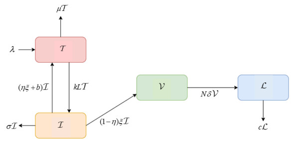
In this paper, we apply the fractal-fractional derivative in the Atangana-Baleanu sense to a model of the human immunodeficiency virus infection of CD$ 4^{+} $ T-cells in the presence of a reverse transcriptase inhibitor, which occurs before the infected cell begins producing the virus. The existence and uniqueness results obtained by applying Banach-type and Leray-Schauder-type fixed-point theorems for the solution of the suggested model are established. Stability analysis in the context of Ulam's stability and its various types are investigated in order to ensure that a close exact solution exists. Additionally, the equilibrium points and their stability are analyzed by using the basic reproduction number. Three numerical algorithms are provided to illustrate the approximate solutions by using the Newton polynomial approach, the Adam-Bashforth method and the predictor-corrector technique, and a comparison between them is presented. Furthermore, we present the results of numerical simulations in the form of graphical figures corresponding to different fractal dimensions and fractional orders between zero and one. We analyze the behavior of the considered model for the provided values of input factors. As a result, the behavior of the system was predicted for various fractal dimensions and fractional orders, which revealed that slight changes in the fractal dimensions and fractional orders had no impact on the function's behavior in general but only occur in the numerical simulations.
Citation: Jutarat Kongson, Chatthai Thaiprayoon, Apichat Neamvonk, Jehad Alzabut, Weerawat Sudsutad. Investigation of fractal-fractional HIV infection by evaluating the drug therapy effect in the Atangana-Baleanu sense[J]. Mathematical Biosciences and Engineering, 2022, 19(11): 10762-10808. doi: 10.3934/mbe.2022504
In this paper, we apply the fractal-fractional derivative in the Atangana-Baleanu sense to a model of the human immunodeficiency virus infection of CD$ 4^{+} $ T-cells in the presence of a reverse transcriptase inhibitor, which occurs before the infected cell begins producing the virus. The existence and uniqueness results obtained by applying Banach-type and Leray-Schauder-type fixed-point theorems for the solution of the suggested model are established. Stability analysis in the context of Ulam's stability and its various types are investigated in order to ensure that a close exact solution exists. Additionally, the equilibrium points and their stability are analyzed by using the basic reproduction number. Three numerical algorithms are provided to illustrate the approximate solutions by using the Newton polynomial approach, the Adam-Bashforth method and the predictor-corrector technique, and a comparison between them is presented. Furthermore, we present the results of numerical simulations in the form of graphical figures corresponding to different fractal dimensions and fractional orders between zero and one. We analyze the behavior of the considered model for the provided values of input factors. As a result, the behavior of the system was predicted for various fractal dimensions and fractional orders, which revealed that slight changes in the fractal dimensions and fractional orders had no impact on the function's behavior in general but only occur in the numerical simulations.

| [1] |
G. Haas, A. Hosmalin, F. Hadida, J. Duntze, P. Debre, B. Autran, Dynamics of HIV variants and specific cytotoxic T-cell recognition in nonprogressors and progressors, Immunol. Lett., 57 (1997), 63–68. https://doi.org/10.1016/S0165-2478(97)00076-X doi: 10.1016/S0165-2478(97)00076-X

|
| [2] | F. Kirchhoff, IV life cycle: Overview. In: T. Hope, M. Stevenson, D. Richman, (eds), Encycl. AIDS, Springer, New York, (2013), 1–9. https://doi.org/10.1007/978-1-4614-9610-6_60-1 |
| [3] |
M. A. Nowak, S. Bonhoeffer, G. M. Shaw, R. M. May, Anti-viral drug treatment: Dynamics of resistance in free virus and infected cell populations, J. Theor. Biol., 184 (1997), 203–217. https://doi.org/10.1006/jtbi.1996.0307 doi: 10.1006/jtbi.1996.0307
|
| [4] |
T. B. Kepler, A. S. Perelson, Drug concentration heterogeneity facilitates the evolution of drug resistance, Proc. Natl. Acad. Sci. USA, 95 (1998), 11514–11519. https://doi.org/10.1073/pnas.95.20.11514 doi: 10.1073/pnas.95.20.11514
|
| [5] |
R. J. Smith, L. M. Wahl, Distinct effects of protease and reverse transcriptase inhibition in an immunological model of HIV-1 infection with impulsive drug effects, Bull. Math. Biol., 66 (2004), 1259–1283. https://doi.org/10.1016/j.bulm.2003.12.004 doi: 10.1016/j.bulm.2003.12.004
|
| [6] | T. H. Zha, O. Castillo, H. Jahanshahi, A. Yusuf, M. O. Alassafi, F. E. Alsaadi, et al., A fuzzy-based strategy to suppress the novel coronavirus (2019-NCOV) massive outbreak, Appl. Comput. Math., 20 2021,160–176. |
| [7] |
M. A. Iqbal, Y. Wang, M. M. Miah, M. S. Osman, Study on DateJimbo-Kashiwara-Miwa equation with conformable derivative dependent on time parameter to find the exact dynamic wave solutions, Fractal Fract., 6 (2022), 1–12. https://doi.org/10.3390/fractalfract6010004 doi: 10.3390/fractalfract6010004
|
| [8] | Y. M. Chu, S. Bashir, M. Ramzan, M. Y. Malik, Model-based comparative study of magnetohydrodynamics unsteady hybrid nanofluid flow between two infinite parallel plates with particle shape effects, Math. Methods Appl. Sci., 2022. http://dx.doi.org/10.1002/mma.8234 |
| [9] |
M. Nazeer, F. Hussain, M. I. Khan, A. U. Rehman, E. R. El-Zahar, Y. M. Chu, et al., Theoretical study of MHD electro-osmotically flow of third-grade fluid in micro channel, Appl. Math. Comput., 420 (2022), 126868. https://doi.org/10.1016/j.amc.2021.126868 doi: 10.1016/j.amc.2021.126868
|
| [10] |
Y. M. Chu, B. M. Shankaralingappa, B. J. Gireesha, F. Alzahrani, M. I. Khan, S. U. Khan, Combined impact of Cattaneo-Christov double diffusion and radiative heat flux on bio-convective flow of Maxwell liquid configured by a stretched nanomaterial surface, Appl. Math. Comput., 419 (2022), 126883. https://doi.org/10.1016/j.amc.2021.126883 doi: 10.1016/j.amc.2021.126883
|
| [11] | T. H. Zhao, M. I. Khan, Y. M. Chu, Artificial neural networking (ANN) analysis for heat and entropy generation in flow of non-Newtonian fluid between two rotating disks, Math. Methods Appl. Sci., 2021. https://doi.org/10.1002/mma.7310 |
| [12] |
L. Wang, M. Y. Li, Mathematical analysis of the global dynamics of a model for HIV infection of CD4+ T cells, Math. Biosci., 200 (2006), 44–57. https://doi.org/10.1016/j.mbs.2005.12.026 doi: 10.1016/j.mbs.2005.12.026
|
| [13] |
P. K. Srivastava, M. Banerjee, P. Chandra, Modeling the drug therapy for HIV infection, J. Biol. Syst., 17 (2009), 213–223. https://doi.org/10.1142/S0218339009002764 doi: 10.1142/S0218339009002764
|
| [14] |
A. Dutta, P. K. Gupta, A mathematical model for transmission dynamics of HIV/AIDS with effect of weak CD$4+$ T cells, Chin. J. Phys., 56 (2018), 1045–1056. https://doi.org/10.1016/j.cjph.2018.04.004 doi: 10.1016/j.cjph.2018.04.004
|
| [15] |
L. Rong, M. A. Gilchrist, Z. Feng, A. S. Perelson, Modeling within host HIV-$1$ dynamics and the evolution of drug resistance: Trade offs between viral enzyme function and drug susceptibility, J. Theor. Biol., 247 (2007), 804–818. https://doi.org/10.1016/j.jtbi.2007.04.014 doi: 10.1016/j.jtbi.2007.04.014
|
| [16] |
Z. Mukandavire, C. Chiyaka, W. Garira, G. Musuka, Mathematical analysis of a sex-structured HIV/AIDS model with a discrete time delay, Nonlinear Anal., Theory Methods Appl., 71 (2009), 1082–1093. https://doi.org/10.1016/j.na.2008.11.026 doi: 10.1016/j.na.2008.11.026
|
| [17] |
M. F. Tabassum, M. Saeed, A. Akgül, M. Farman, N. A. Chaudhry, Treatment of HIV/AIDS epidemic model with vertical transmission by using evolutionary Pade-approximation, Chaos Solitons Fractals, 134 (2020), 109686. https://doi.org/10.1016/j.chaos.2020.109686 doi: 10.1016/j.chaos.2020.109686
|
| [18] | A. S. Perelson, Modeling the interaction of the immune system with HIV, In: C. Castillo-Chavez (eds) Mathematical and Statistical Approaches to AIDS Epidemiology, Lecture Notes in Biomathematics, Springer, Berlin, Heidelberg, (1989), 350–370. https://doi.org/10.1007/978-3-642-93454-4_17 |
| [19] |
A. S. Perelson, D. E. Kirschner, R. D. Boer, Dynamics of HIV infection of CD$4+$ T cells, Math. Biosci., 114 (1993), 81–125. https://doi.org/10.1016/0025-5564(93)90043-A doi: 10.1016/0025-5564(93)90043-A
|
| [20] |
S. Arshad, O. Defterli, D. Baleanu, A second order accurate approximation for fractional derivatives with singular and non-singular kernel applied to a HIV model, Appl. Math. Comput., 374 (2020), 125061. https://doi.org/10.1016/j.amc.2020.125061 doi: 10.1016/j.amc.2020.125061
|
| [21] |
D. Baleanu, H. Mohammadi, S. Rezapour, Analysis of the model of HIV-$1$ infection of CD$4+$ T-cell with a new approach of fractional derivative, Adv. Differ. Equation, 2020 (2020), 1–17. https://doi.org/10.1186/s13662-020-02544-w doi: 10.1186/s13662-020-02544-w
|
| [22] |
A. Jan, R. Jan, H. Khan, M. S. Zobaer, R. Shah, Fractional-order dynamics of Rift Valley fever in ruminant host with vaccination, Commun. Math. Biol. Neurosci., 2020 (2020), 1–32. https://doi.org/10.28919/cmbn/5017 doi: 10.28919/cmbn/5017
|
| [23] |
R. Jan, M. A. Khan, P. Kumam, P. Thounthong, Modeling the transmission of dengue infection through fractional derivatives, Chaos, Solitons Fractals, 127 (2019), 189–216. https://doi.org/10.1016/j.chaos.2019.07.002 doi: 10.1016/j.chaos.2019.07.002
|
| [24] |
F. Wang, M. N. Khan, I. Ahmad, H. Ahmad, H. Abu-Zinadah, Y. M. Chu, Numerical solution of traveling waves in chemical kinetics: time fractional fishers equations, Fractals, 30 (2022), 22400051, 1–11. https://doi.org/10.1142/S0218348X22400515 doi: 10.1142/S0218348X22400515
|
| [25] |
Y. M. Chu, A. Ali, M. A. Khan, S. Islam, S. Ullah, Dynamics of fractional order COVID-19 model with a case study of Saudi Arabia, Results Phys., 21 (2021), 103787. https://doi.org/10.1016/j.rinp.2020.103787 doi: 10.1016/j.rinp.2020.103787
|
| [26] |
M. A. Khan, S. Ullah, M. Farhan, The dynamics of Zika virus with Caputo fractional derivative, AIMS Math., 4 (2019), 134–146. https://doi.org/10.3934/Math.2019.1.134 doi: 10.3934/Math.2019.1.134
|
| [27] |
A. Atangana, Fractal-fractional differentiation and integtion: connecting fractal calculus and fractional calculus to predict complex system, Chaos, Solitons Fractals, 102 (2017), 396–406. https://doi.org/10.1016/j.chaos.2017.04.027 doi: 10.1016/j.chaos.2017.04.027
|
| [28] |
S. Bushnaq, S. A. Khan, K. Shah, G. Zaman, Mathematical analysis of HIV/AIDS infection model with Caputo-Fabrizio fractional derivative, Cogent Math. Stat., 5 (2018), 1432521. https://doi.org/10.1080/23311835.2018.1432521 doi: 10.1080/23311835.2018.1432521
|
| [29] |
S. Ahmad, A. Ullah, M. Arfan, K. Shah, On analysis of the fractional mathematical model of rotavirus epidemic with the effects of breastfeeding and vaccination under Atangana Baleanu (AB) derivative, Chaos, Solitons Fractals, 140 (2020), 110233. https://doi.org/10.1016/j.chaos.2020.110233 doi: 10.1016/j.chaos.2020.110233
|
| [30] |
P. A. Naik, M. Yavuz, J. Zu, The role of prostitution on HIV transmission with memory: A modeling approach, Alexandria Eng. J., 59 (2020), 2513–2531. https://doi.org/10.1016/j.aej.2020.04.016 doi: 10.1016/j.aej.2020.04.016
|
| [31] |
Z. Shah, R. Jan, P. Kumam, W. Deebani, M. Shutaywi, Fractional dynamics of HIV with source term for the supply of new CD4+ T-cells depending on the viral load via Caputo-Fabrizio derivative, Molecules, 26 (2021), 1806. https://doi.org/10.3390/molecules26061806 doi: 10.3390/molecules26061806
|
| [32] |
J. Kongson, C. Thaiprayoon, W. Sudsutad, Analysis of a fractional model for HIV CD$4+$ T-cells with treatment under generalized Caputo fractional derivative, AIMS Math., 6 (2021), 7285–7304. https://doi.org/10.3934/math.2021427 doi: 10.3934/math.2021427
|
| [33] |
Fatmawati, M. A. Khan, The dynamics of dengue in fection through fractal-fractional operator with real statistical data, Alexandria Eng. J., 60 (2021), 321–336. https://doi.org/10.1016/j.aej.2020.08.018 doi: 10.1016/j.aej.2020.08.018
|
| [34] | P. A. Naik, M. Ghoreishi, J. Zu, Approximate solution of a nonlinear fractional-order HIV model using homotopy analysis method, Int. J. Numer. Anal. Mod., 19 (2022), 52–84. |
| [35] |
D. Baleanu, A. Jajarmi, H. Mohammadi, S. Rezapour, A new study on the mathematical modelling of human liver with Caputo-Fabrizio fractional derivative, Chaos Solitons Fractals, 134 (2020), 109705. https://doi.org/10.1016/j.chaos.2020.109705 doi: 10.1016/j.chaos.2020.109705
|
| [36] |
E. Uçara, N. Özdemir, A fractional model of cancer-immune system with Caputo and Caputo-Fabrizio derivatives, Eur. Phys. J. Plus, 136 (2021), 1–17. https://doi.org/10.1140/epjp/s13360-020-00966-9 doi: 10.1140/epjp/s13360-020-00966-9
|
| [37] |
Z. Ali, F. Rabiei, K. Shah, T. Khodadadi, Fractal-fractional order dynamical behavior of an HIV/AIDS epidemic mathematical model, Eur. Phys. J. Plus, 136 (2021), 1–17. https://doi.org/10.1140/epjp/s13360-020-00994-5 doi: 10.1140/epjp/s13360-020-00994-5
|
| [38] | S. Ahmad, A. Ullah, A. Akgül, M. D. L. Sen, Study of HIV disease and its association with immune cells under nonsingular and nonlocal fractal-fractional operator, Alexandria Eng. J., (2021), 1904067. https://doi.org/10.1155/2021/1904067 |
| [39] |
P. A. Naik, J. Zu, K. M. Owolabi, Modeling the mechanics of viral kinetics under immune control during primary infection of HIV-$1$ with treatment in fractional order, Phys. A: Stat. Mech. Appl., 545 (2020), 123816. https://doi.org/10.1016/j.physa.2019.123816 doi: 10.1016/j.physa.2019.123816
|
| [40] |
P. A. Naik, K. M. Owolabi, M. Yavuz, J. Zu, Chaotic dynamics of a fractional order HIV-$1$ model involving AIDS-related cancer cells, Chaos, Solitons Fractals, 140 (2020), 110272. https://doi.org/10.1016/j.chaos.2020.110272 doi: 10.1016/j.chaos.2020.110272
|
| [41] |
P. A. Naik, J. Zu, M. Ghoreishi, Estimating the approximate analytical solution of HIV viral dynamic model by using homotopy analysis method, Chaos, Solitons Fractals, 131 (2020), 109500. https://doi.org/10.1016/j.chaos.2019.109500 doi: 10.1016/j.chaos.2019.109500
|
| [42] | M. M. El-Dessoky, M. A. Khan, Modeling and analysis of an epidemic model with fractal-fractional Atangana-Baleanu derivative, Alexandria Eng. J., 61 (2022), 729–746. https://doi.org/10.1016/j.aej.2021.04.103 |
| [43] | X. Q. Zhao, The theory of basic reproduction ratios, in Dynamical Systems in Population Biology, CMS Books in Mathematics, Springer, Cham, (2017), 285–315. https://doi.org/10.1007/978-3-319-56433-3_11 |
| [44] | C. Castillo-Chavez, Z. Feng, W. Huang, On the computation of $R_0$ and its role on global stability, in Mathematical Approaches for Emerging and Reemerging Infectious Diseases: An Introduction, Springer, Berlin, 2002. https://doi.org/10.1007/978-1-4757-3667-0_13 |
| [45] |
E. Ahmeda, A. S. Elgazzar, On fractional order differential equations model for nonlocal epidemics, Phys. A: Stat. Mech. Appl., 379 (2007), 607–614. https://doi.org/10.1016/j.physa.2007.01.010 doi: 10.1016/j.physa.2007.01.010
|
| [46] |
S. Bourafaa, M. S. Abdelouahaba, A. Moussaoui, On some extended Routh–Hurwitz conditions for fractional-order autonomous systems of order $\alpha \in (0, 2)$ and their applications to some population dynamic models, Chaos, Solitons Fractals, 133 (2020), 109623. https://doi.org/10.1016/j.chaos.2020.109623 doi: 10.1016/j.chaos.2020.109623
|
| [47] | A. Granas, J. Dugundji, Fixed Point Theory, Springer, New York, 2003. https://doi.org/10.1007/978-0-387-21593-8 |
| [48] | D. H. Griffel, Applied Functional Analysis, Ellis Horwood: Chichester, UK, 1981. |
| [49] | A. Atangana, S. I. Araz, New Numerical Scheme with Newton Polynomial: Theory, Methods, and Applications, 1st edition, Elsevier, 2021. https://doi.org/10.1016/C2020-0-02711-8 |
| [50] |
A. T. Haase, K. Henry, M. Zupancic, G. Sedgewick, R. A. Faust, H. Melroe, et al., Quantitative image analysis of HIV-1 infection in lymphoid tissue, Science, 274 (1996), 985–989. https://doi.org/10.1126/science.274.5289.9 doi: 10.1126/science.274.5289.9
|
| [51] |
R. D. Hockett, J. M. Kilby, C. A. Derdeyn, M. S. Saag, M. Sillers, K. Squires, et al., Constant mean viral copy number per infected cell in tissues regardless of high, low, or undetectable plasma HIV RNA, J. Exp. Med., 189 (1999), 1545–1554. https://doi.org/10.1084/jem.189.10.1545 doi: 10.1084/jem.189.10.1545
|
| [52] |
P. Essunger, A. S. Perelson, Modeling HIV infection of CD$4^+$ T-cell subpopulations, J. Theor. Biol., 170 (1994), 367–391. https://doi.org/10.1006/jtbi.1994.1199 doi: 10.1006/jtbi.1994.1199
|
| [53] |
H. Mohri, S. Bonhoeffer, S. Monard, A. S. Perelson, D. D. Ho, Rapid turnover of T lymphocytes in SIV-infected rhesus macaques, Science, 279 (1998), 1223–1227. https://doi.org/10.1126/science.279.5354.1223 doi: 10.1126/science.279.5354.1223
|


Figures(17) / Tables(7)

Jutarat Kongson, Chatthai Thaiprayoon, Apichat Neamvonk, Jehad Alzabut, Weerawat Sudsutad. Investigation of fractal-fractional HIV infection by evaluating the drug therapy effect in the Atangana-Baleanu sense[J]. Mathematical Biosciences and Engineering, 2022, 19(11): 10762-10808. doi: 10.3934/mbe.2022504


 DownLoad: