Optimal harvesting for a periodic $ n $-dimensional food chain model with size structure in a polluted environment

Tainian Zhang; Zhixue Luo; Hao Zhang; Tainian Zhang; Zhixue Luo; Hao Zhang

doi:10.3934/mbe.2022352

Mathematical Biosciences and Engineering

2022, Volume 19, Issue 8: 7481-7503. doi: 10.3934/mbe.2022352

Previous Article Next Article

Research article

Optimal harvesting for a periodic $ n $-dimensional food chain model with size structure in a polluted environment

1.
School of Environmental and Municipal Engineering, Lanzhou Jiaotong University, Lanzhou 730070, China
2.
School of Mathematics and Physics, Lanzhou Jiaotong University, Lanzhou 730070, China

Academic Editor: Hermann J. Eberl

Received: 12 March 2022 Revised: 19 April 2022 Accepted: 02 May 2022 Published: 19 May 2022

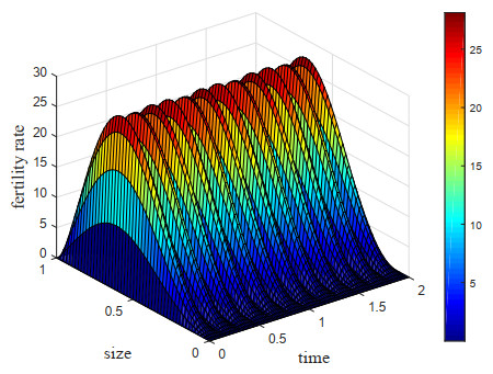
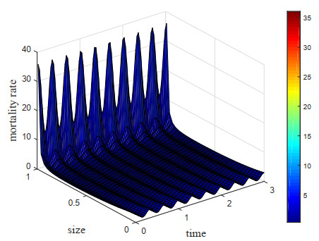
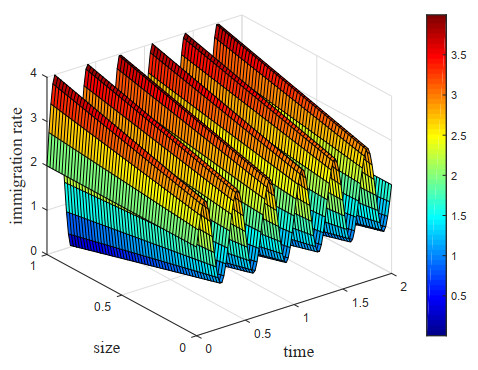
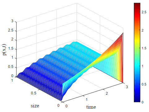
This study examines an optimal harvesting problem for a periodic $ n $-dimensional food chain model that is dependent on size structure in a polluted environment. This is closely related to the protection of biodiversity, as well as the development and utilization of renewable resources. The model contains state variables representing the density of the $ i $th population, the concentration of toxicants in the $ i $th population, and the concentration of toxicants in the environment. The well-posedness of the hybrid system is proved by using the fixed point theorem. The necessary optimality conditions are derived by using the tangent-normal cone technique in nonlinear functional analysis. The existence and uniqueness of the optimal control pair are verified via the Ekeland variational principle. The finite difference scheme and the chasing method are used to approximate the nonnegative T-periodic solution of the state system corresponding to a given initial datum. Some numerical tests are given to illustrate that the numerical solution has good periodicity. The objective functional here represents the total profit obtained from harvesting $ n $ species.
- food chain model,
- size structure,
- optimal harvesting,
- pollution,
- finite difference method
Citation: Tainian Zhang, Zhixue Luo, Hao Zhang. Optimal harvesting for a periodic $ n $-dimensional food chain model with size structure in a polluted environment[J]. Mathematical Biosciences and Engineering, 2022, 19(8): 7481-7503. doi: 10.3934/mbe.2022352

Related Papers:

Abstract

This study examines an optimal harvesting problem for a periodic $ n $-dimensional food chain model that is dependent on size structure in a polluted environment. This is closely related to the protection of biodiversity, as well as the development and utilization of renewable resources. The model contains state variables representing the density of the $ i $th population, the concentration of toxicants in the $ i $th population, and the concentration of toxicants in the environment. The well-posedness of the hybrid system is proved by using the fixed point theorem. The necessary optimality conditions are derived by using the tangent-normal cone technique in nonlinear functional analysis. The existence and uniqueness of the optimal control pair are verified via the Ekeland variational principle. The finite difference scheme and the chasing method are used to approximate the nonnegative T-periodic solution of the state system corresponding to a given initial datum. Some numerical tests are given to illustrate that the numerical solution has good periodicity. The objective functional here represents the total profit obtained from harvesting $ n $ species.

References

[1]	T. G. Hallam, C. E. Clark, R. R. Lassiter, Effects of toxicants on populations: A qualitative approach I. Equilibrium environmental exposure, Ecol. Modell., 18 (1983), 291–304. https://doi.org/10.1016/0304-3800(83)90019-4 doi: 10.1016/0304-3800(83)90019-4
[2]	T. G. Hallam, C. E. Clark, G. S. Jordan, Effects of toxicants on populations: A qualitative approach Ⅱ. First order kinetics, J. Math. Biol., 18 (1983), 25–37. https://doi.org/10.1007/BF00275908 doi: 10.1007/BF00275908
[3]	T. G. Hallam, J. T. De Luna, Effects of toxicants on populations: A qualitative approach Ⅲ. Environmental and food chain pathways, J. Theor. Biol., 109 (1984), 411–429. https://doi.org/10.1016/S0022-5193(84)80090-9 doi: 10.1016/S0022-5193(84)80090-9
[4]	Z. X. Luo, Z. R. He, Optimal control of age-dependent population hybrid system in a polluted environment, Appl. Math. Comput., 228 (2014), 68–76. http://dx.doi.org/10.1016/j.amc.2013.11.070 doi: 10.1016/j.amc.2013.11.070
[5]	Z. X. Luo, X. L. Fan, Optimal control of an age-dependent competitive species model in a polluted environment, Appl. Math. Comput., 228 (2014), 91–101. http://dx.doi.org/10.1016/j.amc.2013.11.069 doi: 10.1016/j.amc.2013.11.069
[6]	Z. X. Luo, Optimal control of an age-dependent predator-prey system in a polluted environment, J. Appl. Math. Comput., 228 (2014), 91–101. https://doi.org/10.1007/s12190-013-0704-y doi: 10.1007/s12190-013-0704-y
[7]	M. Liu, C. X. Du, M. L. Deng, Persistence and extinction of a modified Leslie-Gower Holling-type Ⅱ stochastic predator-prey model with impulsive toxicant input in polluted environments, Nonlinear Anal. Hybrid Syst., 27 (2018), 177–190. http://dx.doi.org/10.1016/j.nahs.2017.08.001 doi: 10.1016/j.nahs.2017.08.001
[8]	X. He, M. J. Shan, M. Liu, Persistence and extinction of an $n$-species mutualism model with random perturbations in a polluted environment, Physica A, 491 (2018), 313–424. http://dx.doi.org/10.1016/j.physa.2017.08.083 doi: 10.1016/j.physa.2017.08.083
[9]	H. Wang, F. M. Pan, M. Liu, Survival analysis of a stochastic service-resource mutualism model in a polluted environment with pulse toxicant input, Physica A, 521 (2019), 591–606. https://doi.org/10.1016/j.physa.2019.01.108 doi: 10.1016/j.physa.2019.01.108
[10]	N. Hritonenko, Y. Yatsenko, R. U. Goetz, A. Xabadia, A bang-bang regime in optimal harvesting of size-structured populations, Nonlinear Anal., 71 (2009), 2331–2336. https://doi.org/10.1016/j.na.2009.05.070 doi: 10.1016/j.na.2009.05.070
[11]	N. Kato, Optimal harvesting for nonlinear size-structured population dynamics, J. Math. Anal. Appl., 342 (2008), 1388–1398. https://doi.org/10.1016/j.jmaa.2008.01.010 doi: 10.1016/j.jmaa.2008.01.010
[12]	R. Liu, G. R. Liu, Optimal birth control problems for a nonlinear vermin population model with size-structure, J. Math. Anal. Appl., 449 (2017), 265–291. http://dx.doi.org/10.1016/j.jmaa.2016.12.010 doi: 10.1016/j.jmaa.2016.12.010
[13]	R. Liu, G. R. Liu, Optimal contraception control fora nonlinear vermin population model with size-structure, Appl. Math. Optim., 79 (2019), 231–256. https://doi.org/10.1007/s00245-017-9428-y doi: 10.1007/s00245-017-9428-y
[14]	Z. R. He, Y. Liu, An optimal birth control problem for a dynamical population model with size-structure, Nonlinear Anal. Real World Appl., 13 (2012), 1369–1378. https://doi.org/10.1016/j.nonrwa.2011.11.001 doi: 10.1016/j.nonrwa.2011.11.001
[15]	Y. Liu, Z. R. He, Behavioral analysis of a nonlinear three-staged population model with age-size-structure, Appl. Math. Comput., 227 (2014), 437–448. http://dx.doi.org/10.1016/j.amc.2013.11.064 doi: 10.1016/j.amc.2013.11.064
[16]	J. Liu, X. S. Wang, Numerical optimal control of a size-structured PDE model for metastatic cancer treatment, Math. Biosci., 314 (2019), 28–42. https://doi.org/10.1016/j.mbs.2019.06.001 doi: 10.1016/j.mbs.2019.06.001
[17]	Y. J. Li, Z. H. Zhang, Y. F. Lv, Z. Liu, Optimal harvesting for a size-stage-structured population model, Nonlinear Anal. Real World Appl., 44 (2018), 616–630. https://doi.org/10.1016/j.nonrwa.2018.06.001 doi: 10.1016/j.nonrwa.2018.06.001
[18]	F. Mansal, N. Sene, Analysis of fractional fishery model with reserve area in the context of time-fractional order derivative, Chaos Solitons Fractals, 140 (2020), 110200. https://doi.org/10.1016/j.chaos.2020.110200 doi: 10.1016/j.chaos.2020.110200
[19]	A. Thiao, N. Sene, Fractional optimal economic control problem described by the generalized fractional order derivative, CMES 2019, 1111 (2020), 36–48. https://doi.org/10.1007/978-3-030-39112-6_3 doi: 10.1007/978-3-030-39112-6_3
[20]	Y. Liu, X. L. Cheng, Z. R. He, On the optimal harvesting of size-structured population dynamics, Appl. Math. J. Chin. Univ., 28 (2013), 173–186. https://doi.org/10.1007/s11766-013-2965-5 doi: 10.1007/s11766-013-2965-5
[21]	Z. R. He, R. Liu, Theory of optimal harvesting for a nonlinear size-structured population in periodic environments, Int. J. Biomath., 7 (2014), 1450046. https://doi.org/10.1142/S1793524514500466 doi: 10.1142/S1793524514500466
[22]	F. Q. Zhang, R. Liu, Y. M. Chen, Optimal harvesting in a periodic food chain model with size structures in predators, Appl. Math. Optim., 75 (2017), 229–251. https://doi.org/10.1007/s00245-016-9331-y doi: 10.1007/s00245-016-9331-y
[23]	Z. X. Luo, Z. R. He, W. T. Li, Optimal birth control for an age-dependent $n$-dimensional food chain model, J. Math. Anal. Appl., 287 (2003), 557–576. https://doi.org/10.1016/S0022-247X(03)00569-9 doi: 10.1016/S0022-247X(03)00569-9
[24]	Z. E. Ma, G. R. Cui, W. D. Wang, Persistence and extinction of a population in a polluted environment, Math. Biosci., 101 (1990), 75–97. https://doi.org/10.1016/0025-5564(90)90103-6 doi: 10.1016/0025-5564(90)90103-6
[25]	V. Barbu, Mathematical Methods in Optimization of Differential Systems, Kluwer Academic Publishers, Dordrecht, 1994.
[26]	S. Aniţa, Analysis and Control of Age-Dependent Population Dynamics, Kluwer Academic Publishers, Dordrecht, 2000.

Reader Comments

Your name:*

Email:*
© 2022 the Author(s), licensee AIMS Press. This is an open access article distributed under the terms of the Creative Commons Attribution License (http://creativecommons.org/licenses/by/4.0)