A seven-gene prognostic model related to immune checkpoint PD-1 revealing overall survival in patients with lung adenocarcinoma

Wei Niu; Lianping Jiang; Wei Niu; Lianping Jiang

doi:10.3934/mbe.2021307

Mathematical Biosciences and Engineering

2021, Volume 18, Issue 5: 6136-6154. doi: 10.3934/mbe.2021307

Previous Article Next Article

Research article Special Issues

A seven-gene prognostic model related to immune checkpoint PD-1 revealing overall survival in patients with lung adenocarcinoma

Wei Niu ^,,
Lianping Jiang

Department of Chemotherapy, Fudan University Shanghai Cancer Center, Minhang Branch, Shanghai 200240, China

Academic Editor:Xiangtao Li

Received: 26 April 2021 Accepted: 23 June 2021 Published: 13 July 2021

Background
We aimed to identify the immune checkpoint Programmed cell death 1 (PD-1)-related gene signatures to predict the overall survival of lung adenocarcinoma (LUAD).

Methods
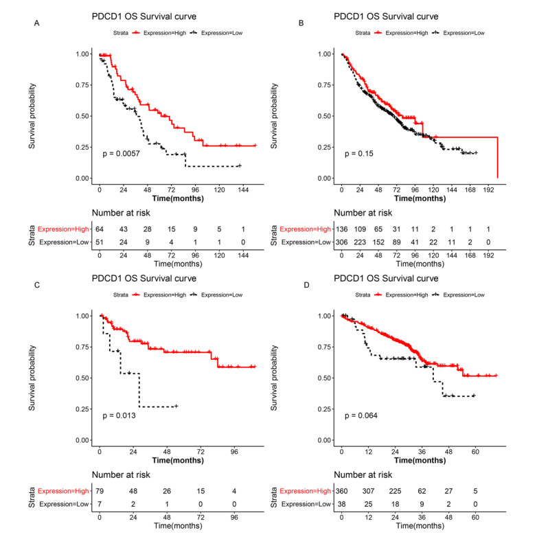
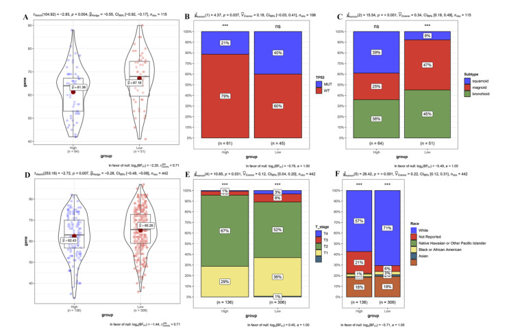
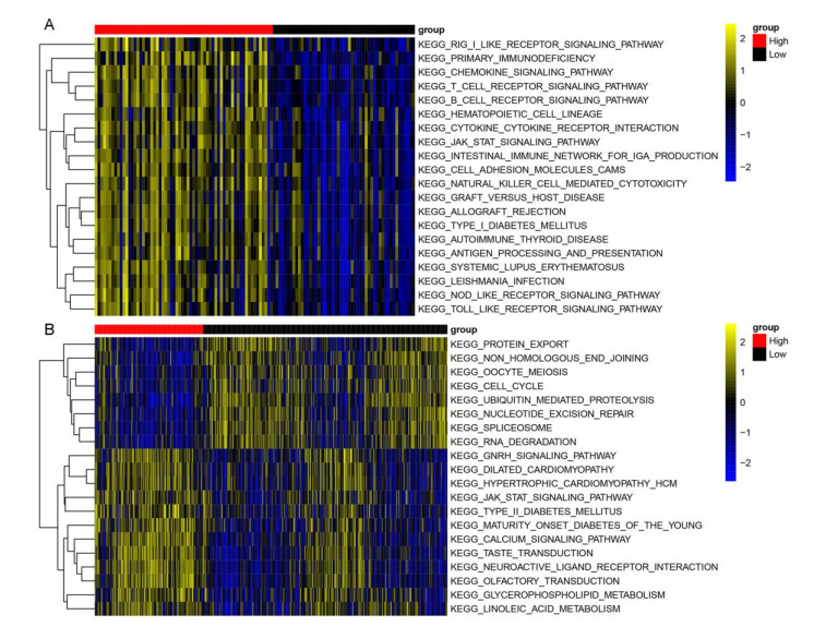
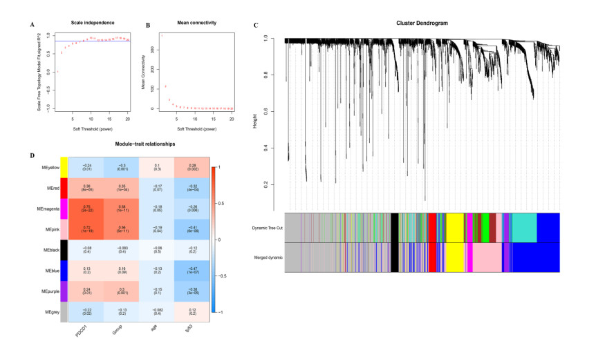
RNA-seq datasets associated with LUAD as well as clinical information were downloaded from the Gene Expression Omnibus (GEO) and The Cancer Genome Atlas (TCGA) databases. Based on the expression level of PD-1, Kaplan-Meier (K-M) survival analysis was performed to divide samples into PD-1 high- and low- expression groups. Then, differentially expressed genes (DEGs) between high- and low- expression groups were identified. Meanwhile, samples were divided into the high and low immune infiltration groups according to score of immune cell, followed by screening of DEGs between these two groups. Subsequently, DEGs related to both PD-1 expression and immune infiltration was integrated to obtain the overlapping genes. Lasso COX regressions were implemented to construct prognostic signatures. The prognostic model was validated using an independent GEO dataset and TCGA cohorts. In addition, the predictive ability of the seven-gene prognostic model with other molecular biomarkers was compared.

Results
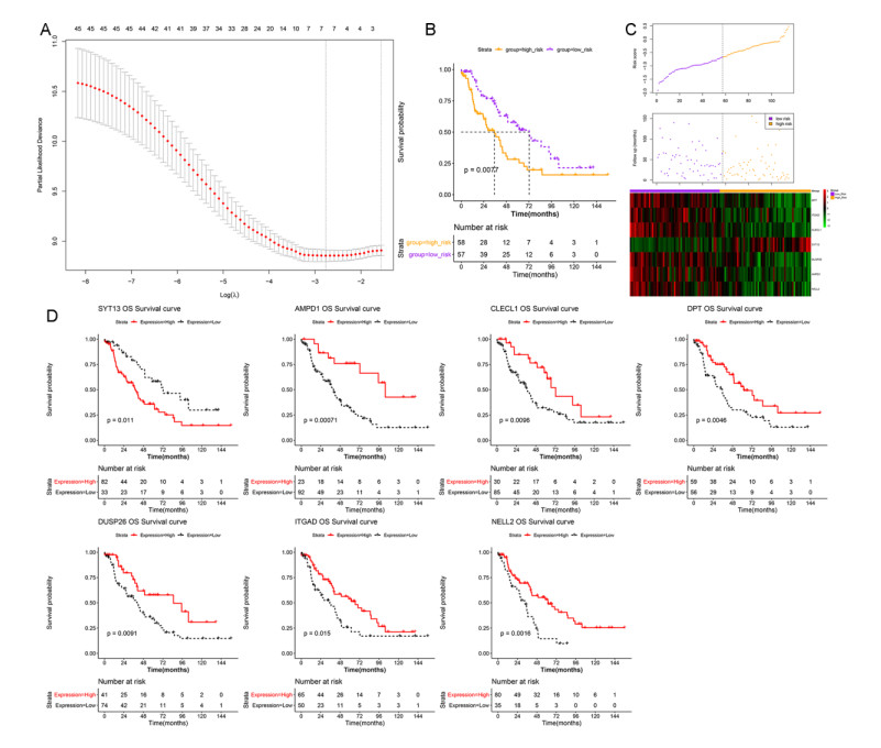
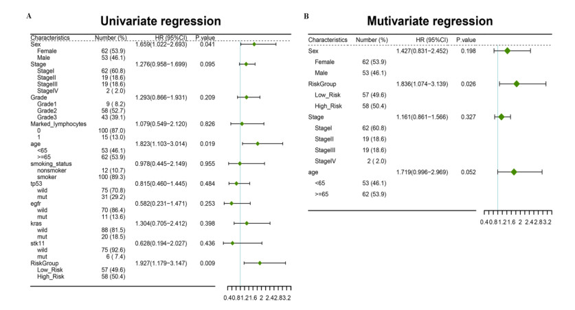
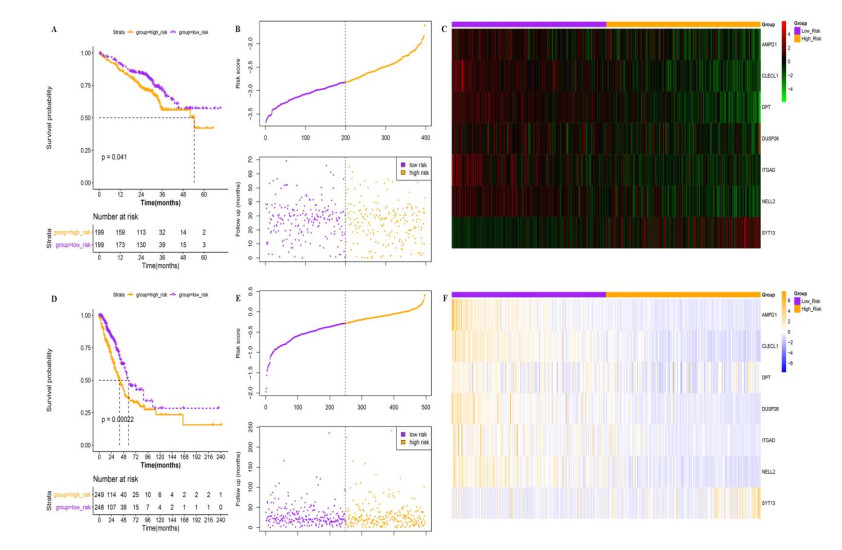
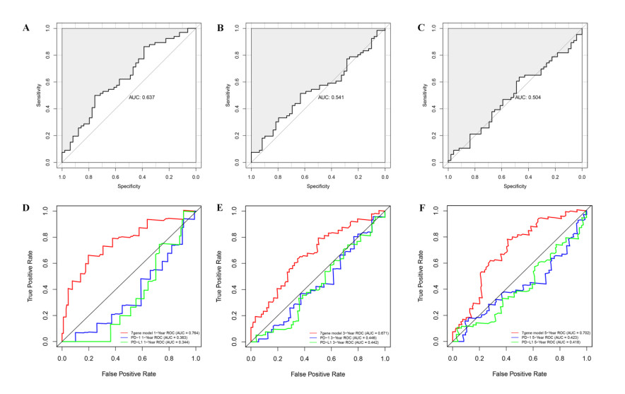
A seven-gene signature (DPT, ITGAD, CLECL1, SYT13, DUSP26, AMPD1, and NELL2) related to PD-1 was developed through Lasso Cox regression. Univariate and multivariate regression analyses indicated that the constructed risk model was an independent prognostic factor. K-M survival analysis indicated that patients in the high risk group had significantly worse prognosis than those in the low risk group. Further, the results of validation analysis showed that this model was reliable and effective.

Conclusions
The constructed prognostic model can predict overall survival in LUAD patients with great predictive performance, and it may be applied for diagnosis and adjuvant treatment of LUAD in clinical trials.
- lung adenocarcinoma,
- programmed cell death 1,
- prognostic model,
- immune infiltration
Citation: Wei Niu, Lianping Jiang. A seven-gene prognostic model related to immune checkpoint PD-1 revealing overall survival in patients with lung adenocarcinoma[J]. Mathematical Biosciences and Engineering, 2021, 18(5): 6136-6154. doi: 10.3934/mbe.2021307

Related Papers:

Abstract

Background

We aimed to identify the immune checkpoint Programmed cell death 1 (PD-1)-related gene signatures to predict the overall survival of lung adenocarcinoma (LUAD).

Methods

RNA-seq datasets associated with LUAD as well as clinical information were downloaded from the Gene Expression Omnibus (GEO) and The Cancer Genome Atlas (TCGA) databases. Based on the expression level of PD-1, Kaplan-Meier (K-M) survival analysis was performed to divide samples into PD-1 high- and low- expression groups. Then, differentially expressed genes (DEGs) between high- and low- expression groups were identified. Meanwhile, samples were divided into the high and low immune infiltration groups according to score of immune cell, followed by screening of DEGs between these two groups. Subsequently, DEGs related to both PD-1 expression and immune infiltration was integrated to obtain the overlapping genes. Lasso COX regressions were implemented to construct prognostic signatures. The prognostic model was validated using an independent GEO dataset and TCGA cohorts. In addition, the predictive ability of the seven-gene prognostic model with other molecular biomarkers was compared.

Results

A seven-gene signature (DPT, ITGAD, CLECL1, SYT13, DUSP26, AMPD1, and NELL2) related to PD-1 was developed through Lasso Cox regression. Univariate and multivariate regression analyses indicated that the constructed risk model was an independent prognostic factor. K-M survival analysis indicated that patients in the high risk group had significantly worse prognosis than those in the low risk group. Further, the results of validation analysis showed that this model was reliable and effective.

Conclusions

The constructed prognostic model can predict overall survival in LUAD patients with great predictive performance, and it may be applied for diagnosis and adjuvant treatment of LUAD in clinical trials.

References

[1]	K. C. Arbour, G. J. Riely, Systemic therapy for locally advanced and metastatic non‑small cell lung cancer, JAMA, 322 (2019), 764-774. doi: 10.1001/jama.2019.11058
[2]	L. Li, T. Feng, J. Qu, N. Feng, Y. Wang, R. Ma, et al., LncRNA expression signature in prediction of the prognosis of lung adenocarcinoma, Genet. Test. Mol. Biomarkers, 22 (2018), 20-28. doi: 10.1089/gtmb.2017.0194
[3]	W. D. Travis, E. Brambilla, A. G. Nicholson, Y. Yatabe, J. H. M. Austin, M. B. Beasley, et al., The 2015 World Health Organization classification of lung tumors: impact of genetic, clinical and radiologic advances since the 2004 classification, J. Thorac. Oncol., 10 (2015), 1243-1260.
[4]	G. S. Lu, M. Li, C. X. Xu, D. Wang, APE1 stimulates EGFR-TKI resistance by activating Akt signaling through a redox-dependent mechanism in lung adenocarcinoma, Cell Death Dis., 9 (2018), 1111. doi: 10.1038/s41419-018-1162-0
[5]	R. L. Siegel, K. D. Miller, A. Jemal, Cancer statistics, 2019, CA Cancer J. Clin., 69 (2019), 7-34. doi: 10.3322/caac.21551
[6]	M. Kieler, M. Unseld, D. Bianconi, G. Prager, Challenges and perspectives for immunotherapy in adenocarcinoma of the pancreas: the cancer immunity cycle, Pancreas, 47(2018), 142-157. doi: 10.1097/MPA.0000000000000970
[7]	A. Mishra, M. Verma, Epigenetic and genetic regulation of PDCD1 gene in cancer immunology, Methods Mol. Biol., 1856 (2018), 247-254. doi: 10.1007/978-1-4939-8751-1_14
[8]	A. O. Kamphorst, R. Ahmed, Manipulating the PD-1 pathway to improve immunity-sciencedirect, Curr. Opin. Immunol., 25 (2013), 381-388. doi: 10.1016/j.coi.2013.03.003
[9]	M. Cai, X. Zhao, M. Cao, P. Ma, M. Chen, J. Wu, et al., T-cell exhaustion interrelates with immune cytolytic activity to shape the inflamed tumor microenvironment, J. Pathol., 251 (2020), 147-159.
[10]	H. Kagamu, K. Kaira, Efficacy of PD-1 blockade therapy and T cell immunity in lung cancer patients, Immunol. Med., 43 (2020), 10-15. doi: 10.1080/25785826.2019.1710427
[11]	Z. Kai, L. Zulei, T. Hui, Twenty-gene-based prognostic model predicts lung adenocarcinoma survival, Onco Targets Ther., 11 (2018), 3415. doi: 10.2147/OTT.S158638
[12]	W. Zhang, Y. Shen, G. Feng, Predicting the survival of patients with lung adenocarcinoma using a four-gene prognosis risk model, Oncol. Lett., 18 (2019), 535-544.
[13]	S. Sun, W. Guo, Z. Wang, X. Wang, G. Zhang, H. Zhang, et al., Development and validation of an immune-related prognostic signature in lung adenocarcinoma, Cancer Med., 9 (2020), 5960-5975. doi: 10.1002/cam4.3240
[14]	T. Barrett, T. O. Suzek, D. B. Troup, S. E. Wilhite, W. C. Ngau, P. Ledoux, et al., NCBI GEO: mining millions of expression profiles-database and tools, Nucleic Acids Res., 33 (2005), D562-566.
[15]	S. Hnzelmann, R. Castelo, J. Guinney, GSVA: gene set variation analysis for microarray and RNA-Seq data, BMC Bioinf., 14 (2013), 7-7. doi: 10.1186/1471-2105-14-7
[16]	M. E. Ritchie, B. Phipson, D. Wu, Y. Hu, C. W. Law, W. Shi, et al., limma powers differential expression analyses for RNA-sequencing and microarray studies, Nucleic Acids Res., 43 (2015), e47.
[17]	P. Langfelder, S. Horvath, WGCNA: an R package for weighted correlation network analysis, BMC Bioinf., 9 (2008), 559. doi: 10.1186/1471-2105-9-559
[18]	G. Yu, L. G. Wang, Y. Han, Q. Y. He, ClusterProfiler: an R package for comparing biological themes among gene clusters, OMICS, 16 (2012), 284-287. doi: 10.1089/omi.2011.0118
[19]	P. Charoentong, F. Finotello, M. Angelova, C. Mayer, M. Efremova, D. Rieder, et al., Pan-cancer immunogenomic analyses reveal genotype-immunophenotype relationships and predictors of response to checkpoint blockade, Cell Rep., 18 (2017), 248-262. doi: 10.1016/j.celrep.2016.12.019
[20]	S. Hänzelmann, R. Castelo, J. Guinney, GSVA: gene set variation analysis for microarray and RNA-seq data, BMC Bioinf., 14 (2013), 7. doi: 10.1186/1471-2105-14-7
[21]	M. Ashburner, C. A. Ball, J. A. Blake, D. Botstein, J. M. Cherry, Gene ontology: tool for the unification of biology. The gene ontology consortium, Nat. Genet., 25 (2000), 25-29.
[22]	M. Gerlich, S. Neumann, KEGG: Kyoto encyclopedia of genes and genomes, Nucleic Acids Res., 28 (2000), 27-30. doi: 10.1093/nar/28.1.27
[23]	W. Huang, B. T. Sherman, R. A. Lempicki, Systematic and integrative analysis of large gene lists using DAVID bioinformatics resources, Nat. Protoc., 4 (2009), 44-57. doi: 10.1038/nprot.2008.211
[24]	J. Friedman, T. Hastie, R. Tibshirani, Regularization paths for generalized linear models via coordinate descent, J. Stat. software, 33 (2010), 1-22.
[25]	P. Blanche, J. F. Dartigues, H. Jacqmin-Gadda, Estimating and comparing time-dependent areas under receiver operating characteristic curves for censored event times with competing risks, Stat. Med., 32 (2013), 5381-5397. doi: 10.1002/sim.5958
[26]	M. Yamatoji, A. Kasamatsu, Y. Kouzu, H. Koike, Y. Sakamoto, K. Ogawara, et al., Dermatopontin: A potential predictor for metastasis of human oral cancer, Int. J. Cancer, 130 (2012), 2903-2911. doi: 10.1002/ijc.26328
[27]	Y. Guo, H. Li, H. Guan, W. Ke, W. Liang, H. Xiao, et al., Dermatopontin inhibits papillary thyroid cancer cell proliferation through MYC repression, Mol. Cell. Endocrinol., 480 (2018), 122-132.
[28]	X. Li, P. Feng, J. Ou, Z. Luo, C. Zhang, Dermatopontin is expressed in human liver and is downregulated in hepatocellular carcinoma, Biochemistry, 74 (2009), 979-985.
[29]	J. Zhang, J. Y. Huang, Y. N. Chen, F. Yuan, H. Zhang, F. H. Yan, et al., Whole genome and transcriptome sequencing of matched primary and peritoneal metastatic gastric carcinoma, Sci. Rep., 5 (2015), 13750. doi: 10.1038/srep13750
[30]	K. M. Boerkamp, M. van der Kooij, F. G. van Steenbeek, M. E. van Wolferen, M. J. Groot Koerkamp, D. van Leenen, et al., Gene expression profiling of histiocytic sarcomas in a canine model: the predisposed flatcoated retriever dog, PLoS One, 8 (2013), e71094.
[31]	M. Kanda, Y. Kasahara, D. Shimizu, T. Miwa, S. Obika, Amido-bridged nucleic acid-modified antisense oligonucleotides targeting SYT13 to treat peritoneal metastasis of gastric cancer, Mol. Ther. Nucleic Acids, 22 (2020), 791-802. doi: 10.1016/j.omtn.2020.10.001
[32]	J. E. Jahn, D. H. Best, W. B. Coleman, Exogenous expression of synaptotagmin XIII suppresses the neoplastic phenotype of a rat liver tumor cell line through molecular pathways related to mesenchymal to epithelial transition, Exp. Mol. Pathol., 89(2010), 209-216. doi: 10.1016/j.yexmp.2010.09.001
[33]	G. Castellini, L. Lelli, E. Cassioli, V. Ricca, Relationships between eating disorder psychopathology, sexual hormones and sexual behaviours, Mol. Cell. Endocrinol., 497 (2019), 110429.
[34]	L. Zhang, B. Fan, Y. Zheng, Y. Lou, X. Tan, Identification SYT13 as a novel biomarker in lung adenocarcinoma, J. Cell. Biochem., 121 (2020), 963-973. doi: 10.1002/jcb.29224
[35]	E. Y. Won, S. O. Lee, D. H. Lee, D. Lee, K. H. Bae, S. C. Lee, et al., Structural insight into the critical role of the N-terminal region in the catalytic activity of dual-specificity phosphatase 26, PLoS One, 11 (2016), e0162115.
[36]	A. M. Bourgonje, K. Verrijp, J. T. Schepens, A. C. Navis, J. A. Piepers, C. B. Palmen, et al., Comprehensive protein tyrosine phosphatase mRNA profiling identifies new regulators in the progression of glioma, Acta Neuropathol. Commun., 4(2016), 96. doi: 10.1186/s40478-016-0372-x
[37]	W. Yu, I. Imoto, J. Inoue, M. Onda, M. Emi, J. Inazawa, A novel amplification target, DUSP26, promotes anaplastic thyroid cancer cell growth by inhibiting p38 MAPK activity, Oncogene, 26 (2007), 1178-1187. doi: 10.1038/sj.onc.1209899
[38]	E. J. Choi, D. H. Kim, J. G. Kim, D. Y. Kim, J. D. Kim, O. J. Seol, et al., Estrogen-dependent transcription of the NEL-like 2 (NELL2) gene and its role in protection from cell death, J. Biol. Chem., 285 (2010), 25074-25084. doi: 10.1074/jbc.M110.100545
[39]	R. Nakamura, T. Oyama, R. Tajiri, A. Mizokami, M. Namiki, M. Nakamoto, et al., Expression and regulatory effects on cancer cell behavior of NELL1 and NELL2 in human renal cell carcinoma, Cancer Sci., 106 (2015), 656-664. doi: 10.1111/cas.12649
[40]	D. H. Kim, Y. -G. Roh, H. H. Lee, S. -Y. Lee, S. I. Kim, B. J. Lee, et al., The E2F1 oncogene transcriptionally regulates NELL2 in cancer cells, DNA Cell Biol., 32(2013), 517-523.
[41]	H. Lubli, L. Borsig, Altered cell adhesion and glycosylation promote cancer immune suppression and metastasis, Front. Immunol., 10 (2019), 2120. doi: 10.3389/fimmu.2019.02120
[42]	H. Wang, C. E. Rudd, SKAP-55, SKAP-55-related and ADAP adaptors modulate integrin-mediated immune-cell adhesion, Trends Cell Biol., 18 (2008), 486-493. doi: 10.1016/j.tcb.2008.07.005
[43]	R. A. Colvin, T. K. Means, T. J. Diefenbach, L. F. Moita, R. P. Friday, S. Sever, et al., Synaptotagmin-mediated vesicle fusion regulates cell migration, Nat. Immunol., 11 (2010), 495-502. doi: 10.1038/ni.1878
[44]	J. Chen, Z. Wang, W. Wang, S. Ren, C. Zhang, SYT16 is a prognostic biomarker and correlated with immune infiltrates in glioma: A study based on TCGA data, Int. Immunopharmacol., 84 (2020), 106490. doi: 10.1016/j.intimp.2020.106490
[45]	H. B. Low, Y. Zhang, Regulatory roles of MAPK phosphatases in cancer, Immune Netw., 16 (2016), 85-98. doi: 10.4110/in.2016.16.2.85
[46]	H. N. Cukier, B. K. Kunkle, K. L. Hamilton, S. Rolati, M. A. Kohli, P. L. Whitehead, et al., Exome sequencing of extended families with alzheimer's disease identifies novel genes implicated in cell immunity and neuronal function, J. Alzheimers Dis. Parkinsonism, 7 (2017), 355. doi: 10.4172/2161-0460.1000326
[47]	B. P. Ramakers, E. J. Giamarellos-Bourboulis, C. Tasioudis, M. J. Coenen, M. Kox, S. H. Vermeulen, et al., Effects of the 34C > T variant of the AMPD1 gene on immune function, multi-organ dysfunction, and mortality in sepsis patients, Shock, 44 (2015), 542-547.

mbe-18-05-307-Supplementary.pdf

Reader Comments

Your name:*

Email:*
© 2021 the Author(s), licensee AIMS Press. This is an open access article distributed under the terms of the Creative Commons Attribution License (http://creativecommons.org/licenses/by/4.0)