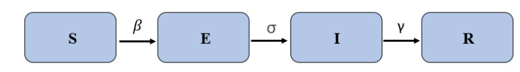
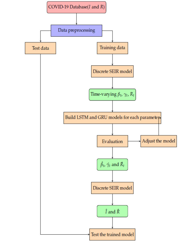
COVID-19 is an infectious disease caused by a newly discovered coronavirus, which has become a worldwide pandemic greatly impacting our daily life and work. A large number of mathematical models, including the susceptible-exposed-infected-removed (SEIR) model and deep learning methods, such as long-short-term-memory (LSTM) and gated recurrent units (GRU)-based methods, have been employed for the analysis and prediction of the COVID-19 outbreak. This paper describes a SEIR-LSTM/GRU algorithm with time-varying parameters that can predict the number of active cases and removed cases in the US. Time-varying reproductive numbers that can illustrate the progress of the epidemic are also produced via this process. The investigation is based on the active cases and total cases data for the USA, as collected from the website "Worldometer". The root mean square error, mean absolute percentage error and $ r_2 $ score were utilized to assess the model's accuracy.
Citation: Lin Feng, Ziren Chen, Harold A. Lay Jr., Khaled Furati, Abdul Khaliq. Data driven time-varying SEIR-LSTM/GRU algorithms to track the spread of COVID-19[J]. Mathematical Biosciences and Engineering, 2022, 19(9): 8935-8962. doi: 10.3934/mbe.2022415
COVID-19 is an infectious disease caused by a newly discovered coronavirus, which has become a worldwide pandemic greatly impacting our daily life and work. A large number of mathematical models, including the susceptible-exposed-infected-removed (SEIR) model and deep learning methods, such as long-short-term-memory (LSTM) and gated recurrent units (GRU)-based methods, have been employed for the analysis and prediction of the COVID-19 outbreak. This paper describes a SEIR-LSTM/GRU algorithm with time-varying parameters that can predict the number of active cases and removed cases in the US. Time-varying reproductive numbers that can illustrate the progress of the epidemic are also produced via this process. The investigation is based on the active cases and total cases data for the USA, as collected from the website "Worldometer". The root mean square error, mean absolute percentage error and $ r_2 $ score were utilized to assess the model's accuracy.

| [1] | BBCnews, Coronavirus disease named COVID-19, 2020. Available from: https://www.bbc.com/news/world-asia-china-51466362. |
| [2] |
S. Roychoudhury, A. Das, P. Sengupta, S. Dutta, S. Roychoudhury, A. P. Choudhury, et al., Viral pandemics of the last four decades: Pathophysiology, health impacts and perspectives, Int. J. Environ. Res. Public Health, 17 (2020), 9411. https://doi.org/10.3390/ijerph17249411 doi: 10.3390/ijerph17249411

|
| [3] | F. Brauer, Compartmental Models in Epidemiology, Springer Berlin Heidelberg, (2008), 19–79. https://doi.org/10.1007/978-3-540-78911-6_2 |
| [4] | F. Salvadore, G. Fiscon, P. Paci, Integro-differential approach for modeling the COVID-19 dynamics-impact of confinement measures in Italy, Comput. Biol. Med., 139 (2021) 105013. https://doi.org/10.1016/j.compbiomed.2021.105013 |
| [5] |
O. Diekmann, J. A. P. Heesterbeek, J. A. J. Metz, On the definition and the computation of the basic reproduction ratio r0 in models for infectious diseases in heterogeneous populations, J. Math. Biol., 28 (1990), 365–382. https://doi.org/10.1007/BF00178324 doi: 10.1007/BF00178324
|
| [6] |
J. M. Heffernan, R. J. Smith, L. M. Wahl, Perspectives on the basic reproductive ratio, J. R. Soc. Interface, 2 (2005), 281–293. https://doi.org/10.1098/rsif.2005.0042 doi: 10.1098/rsif.2005.0042
|
| [7] | R. M. Anderson, R. M. May, Infectious diseases of humans, dynamics and control, Oxford University Press, 1991. |
| [8] |
P. van den Driessche, Reproduction numbers of infectious disease models, Infect. Dis. Model., 2 (2017), 288–303. https://doi.org/doi:doi.org/10.1016/j.idm.2017.06.002 doi: 10.1016/j.idm.2017.06.002
|
| [9] | A. Zeroual, F. Harrou, A. Dairi, Y. Sun, Deep learning methods for forecasting COVID-19 time-series data: A comparative study, Chaos Solitons Fractals, 140 (2020) 110121. https://doi.org/doi.org/10.1016/j.chaos.2020.110121 |
| [10] |
G. Fiscon, F. Salvadore, V. Guarrasi, A. R. Garbuglia, P. Paci, Assessing the impact of data-driven limitations on tracing and forecasting the outbreak dynamics of COVID-19, Comput. Biol. Med., 135 (2021), 104657. https://doi.org/10.1016/j.compbiomed.2021.104657 doi: 10.1016/j.compbiomed.2021.104657
|
| [11] |
S. Bentout, A. Chekroun, T. Kuniya, Parameter estimation and prediction for coronavirus disease outbreak 2019 (COVID-19) in Algeria, AIMS Public Health, 7 (2020), 306–318. https://doi.org/10.3934/publichealth.2020026 doi: 10.3934/publichealth.2020026
|
| [12] |
A. C. S. de Oliveira, L. H. M. Morita, E. B. da Silva, L. A. R. Zardo, C. J. F. Fontes, D. C. T. Granzotto, Bayesian modeling of COVID-19 cases with a correction to account for under-reported cases, Infect. Dis. Model., 5 (2020), 699–713. https://doi.org/10.1016/j.idm.2020.09.005 doi: 10.1016/j.idm.2020.09.005
|
| [13] |
J. Schmidt, M. R. G. Marques, S. Botti, M. A. L. Marques, Recent advances and applications of machine learning in solid-state materials science, NPJ Comput. Materials, 5 (2019), 83. https://doi.org/10.1038/s41524-019-0221-0 doi: 10.1038/s41524-019-0221-0
|
| [14] |
K. Olumoyin, A. Khaliq, K. Furati, Data-driven deep-learning algorithm for asymptomatic COVID-19 model with varying mitigation measures and transmission rate, Epidemiologia, 2 (2021), 471–489. https://doi.org/10.3390/epidemiologia2040033 doi: 10.3390/epidemiologia2040033
|
| [15] |
A. Zeroual, F. Harrou, A. Dairi, Y. Sun, Deep learning methods for forecasting COVID-19 time-series data: A comparative study, Chaos Solitons Fractals, 140 (2020), 110121. https://doi.org/10.1016/j.chaos.2020.110121 doi: 10.1016/j.chaos.2020.110121
|
| [16] |
F. Shahid, A. Zameer, M. Muneeb, Predictions for COVID-19 with deep learning models of lstm, gru and bi-lstm, Chaos Solitons Fractals, 140 (2020), 110212. https://doi.org/10.1016/j.chaos.2020.110212 doi: 10.1016/j.chaos.2020.110212
|
| [17] |
A. Fokas, N. Dikaios, G. Kastis, Mathematical models and deep learning for predicting the number of individuals reported to be infected with Sars-Cov-2, J. R. Soc. Interface, 17 (2020), 20200494. https://doi.org/10.1098/rsif.2020.0494 doi: 10.1098/rsif.2020.0494
|
| [18] |
J. Long, A. Q. M. Khaliq, K. M. Furati, Identification and prediction of time-varying parameters of COVID-19 model: a data-driven deep learning approach, Int. J. Comput. Math., 98 (2021), 1617–1632. https://doi.org/10.1080/00207160.2021.1929942 doi: 10.1080/00207160.2021.1929942
|
| [19] |
B. Ridenhour, J. M. Kowalik, D. K. Shay, Unraveling r0: Considerations for public health applications, Am. J. Public Health, 104 (2014), e32–e41. https://doi.org/10.2105/AJPH.2013.301704 doi: 10.2105/AJPH.2013.301704
|
| [20] |
Z. C. Chen, L. Feng, H. A. L. Lay, K. Furati, A. Khaliq, SEIR model with unreported infected population and dynamic parameters for the spread of COVID-19, Math. Comput. Simul., 198 (2022), 31–46. https://doi.org/10.1016/j.matcom.2022.02.025 doi: 10.1016/j.matcom.2022.02.025
|
| [21] | A. Hassan, I. Shahin, M. B. Alsabek, Covid-19 detection system using recurrent neural networks, in 2020 International Conference on Communications, Computing, Cybersecurity, and Informatics (CCCI), (2020), 1–5. https://doi.org/10.1109/CCCI49893.2020.9256562 |
| [22] | G. Petneházi, Recurrent neural networks for time series forecasting, preprint, arXiv: 1901.00069. |
| [23] |
H. Hewamalage, C. Bergmeir, K. Bandara, Recurrent neural networks for time series forecasting: Current status and future directions, Int. J. Forecast., 37 (2021), 388–427. https://doi.org/10.1016/j.ijforecast.2020.06.008 doi: 10.1016/j.ijforecast.2020.06.008
|
| [24] | S. Hochreiter, J. Schmidhuber, Long short-term memory, Neural Comput., 9 (1997), 1735–1780. https://doi.org/10.1162/neco.1997.9.8.1735 |
| [25] | K. Cho, B. van Merrienboer, C. Gulcehre, D. Bahdanau, F. Bougares, H. Schwenk, et al., Learning phrase representations using rnn encoder-decoder for statistical machine translation, preprint, arXiv: 1406.1078. |
| [26] | Worlometer, Coronavirus cases, 2021. Available from: https://www.worldometers.info/coronavirus/coronavirus-cases/ |
| [27] | S. García, J. Luengo, F. Herrera, Data Preprocessing in Data Mining, Springer International Publishing, (2015), 1–17. https://doi.org/10.1007/978-3-319-10247-4_1 |
| [28] | ProgrammerSought, General process and necessary steps of machine learning tasks, Available from: https://www.programmersought.com/article/98093557423/. |
| [29] | M. Sharma, Data preprocessing: 6 necessary steps for data scientists, Available from: https://hackernoon.com/what-steps-should-one-take-while-doing-data-preprocessing-502c993e1caa. |
| [30] | D. Jain, Data preprocessing in data mining, 2021. Available from: https://www.geeksforgeeks.org/data-preprocessing-in-data-mining/. |
| [31] |
S. B. Kotsiantis, D. Kanellopoulos, P. E. Pintelas, Data preprocessing for supervised learning, Int. J. Comput. Sci., 1 (2006), 111–117. https://doi.org/10.5281/zenodo.1082415 doi: 10.5281/zenodo.1082415
|
| [32] | Centers for Disease Control and Prevention, Symptoms of COVID-19, 2021. Available from: https://www.cdc.gov/coronavirus/2019-ncov/symptoms-testing/symptoms.html. |
| [33] |
S. A. Lauer, K. H. Grantz, Q. Bi, F. K. Jones, Q. Zheng, H. R. Meredith, et al., The incubation period of coronavirus disease 2019 (COVID-19) from publicly reported confirmed cases: Estimation and application, Ann. Intern. Med., 172 (2020), 577–582. https://doi.org/10.7326/M20-0504 doi: 10.7326/M20-0504
|
| [34] |
J. A. Backer, D. Klinkenberg, J. Wallinga, Incubation period of 2019 novel coronavirus (2019-ncov) infections among travellers from Wuhan, China, 20–28 January 2020, Eurosurveillance, 25 (2020), 20–28. https://doi.org/10.2807/1560-7917.ES.2020.25.5.2000062 doi: 10.2807/1560-7917.ES.2020.25.5.2000062
|
| [35] | B. Everitt, A. Skrondal, The Cambridge Dictionary of Statistics, Cambridge University Press, 2010. |
| [36] | S. Glen, Mean absolute percentage error (MAPE), 2021. Available from: https://www.statisticshowto.com/mean-absolute-percentage-error-mape/. |
| [37] | R. G. D. Steel, J. H. Torrie, Principles and procedures of statistics, McGraw-Hill Book Company, 1960. |
| [38] | S. Glantz, B. Slinker, Primer of Applied Regression and Analysis of Variance, McGraw-Hill, 2001. |
| [39] | N. R. Draper, H. Smith, Applied regression analysis, John Wiley and Sons, 1998. |


Figures(15) / Tables(4)

Lin Feng, Ziren Chen, Harold A. Lay Jr., Khaled Furati, Abdul Khaliq. Data driven time-varying SEIR-LSTM/GRU algorithms to track the spread of COVID-19[J]. Mathematical Biosciences and Engineering, 2022, 19(9): 8935-8962. doi: 10.3934/mbe.2022415


 DownLoad: