COVID-19 and underlying health conditions: A modeling investigation

Chayu Yang; Jin Wang; Chayu Yang; Jin Wang

doi:10.3934/mbe.2021191

Mathematical Biosciences and Engineering

2021, Volume 18, Issue 4: 3790-3812. doi: 10.3934/mbe.2021191

Previous Article Next Article

Research article

COVID-19 and underlying health conditions: A modeling investigation

Chayu Yang ¹,
Jin Wang ^{2
,
,}

1.
Department of Mathematics, University of Florida, Gainesville, FL 32607, USA
2.
Department of Mathematics, University of Tennessee at Chattanooga, 615 McCallie Ave., Chattanooga, TN 37403, USA

Academic Editor: Yang Kuang

Received: 07 March 2021 Accepted: 20 April 2021 Published: 30 April 2021

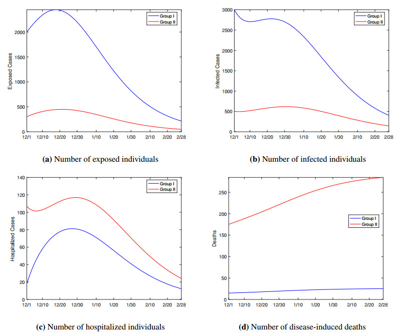
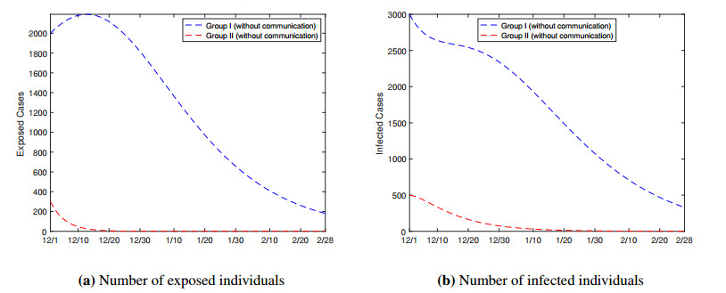
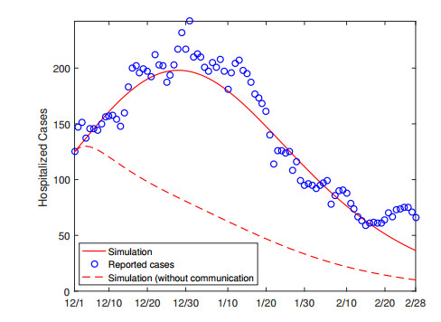
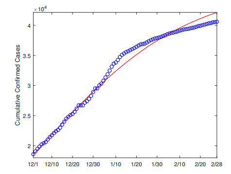
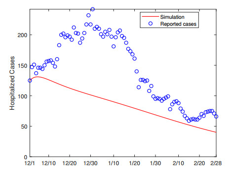
We propose a mathematical model based on a system of differential equations, which incorporates the impact of the chronic health conditions of the host population, to investigate the transmission dynamics of COVID-19. The model divides the total population into two groups, depending on whether they have underlying conditions, and describes the disease transmission both within and between the groups. As an application of this model, we perform a case study for Hamilton County, the fourth-most populous county in the US state of Tennessee and a region with high prevalence of chronic conditions. Our data fitting and simulation results quantify the high risk of COVID-19 for the population group with underlying health conditions. The findings suggest that weakening the disease transmission route between the exposed and susceptible individuals, including the reduction of the between-group contact, would be an effective approach to protect the most vulnerable people in this population group.
- COVID-19 transmission,
- chronic conditions,
- data fitting
Citation: Chayu Yang, Jin Wang. COVID-19 and underlying health conditions: A modeling investigation[J]. Mathematical Biosciences and Engineering, 2021, 18(4): 3790-3812. doi: 10.3934/mbe.2021191

Related Papers:

Abstract

We propose a mathematical model based on a system of differential equations, which incorporates the impact of the chronic health conditions of the host population, to investigate the transmission dynamics of COVID-19. The model divides the total population into two groups, depending on whether they have underlying conditions, and describes the disease transmission both within and between the groups. As an application of this model, we perform a case study for Hamilton County, the fourth-most populous county in the US state of Tennessee and a region with high prevalence of chronic conditions. Our data fitting and simulation results quantify the high risk of COVID-19 for the population group with underlying health conditions. The findings suggest that weakening the disease transmission route between the exposed and susceptible individuals, including the reduction of the between-group contact, would be an effective approach to protect the most vulnerable people in this population group.

References

[1]	Centers for Disease Control and Prevention, Coronavirus (COVID-19). Available from: https://www.cdc.gov/coronavirus/2019-ncov.
[2]	World Health Organization, Coronavirus disease (COVID-19) pandemic. Available from: https://www.who.int/emergencies/diseases/novel-coronavirus-2019.
[3]	A. Clark, M. Jit, C. Warren-Gash, B. Guthrie, H. H. X. Wang, S. W. Mercer, et al., Global, regional, and national estimates of the population at increased risk of severe COVID-19 due to underlying health conditions in 2020: A modelling study, Lancet Glob. Health, 8 (2020), e1003–e1017. doi: 10.1016/S2214-109X(20)30264-3
[4]	E. K. Stokes, L. D. Zambrano, K. N. Anderson, E. P. Marder, K. M. Raz, S. E. B. Felix, et al., Coronavirus disease 2019 case surveillance – United States, January 22–May 30, 2020, Morb. Mortal. Wkly. Rep., 69 (2020), 759-765. doi: 10.15585/mmwr.mm6924e2
[5]	H. Razzaghi, Y. Wang, H. Lu, K. E. Marshall, N. F. Dowling, G. Paz-Bailey, et al., Estimated county-level prevalence of selected underlying medical conditions associated with increased risk for severe COVID-19 illness – United States, 2018, Morb. Mortal. Wkly. Rep., 69 (2020), 945–950. doi: 10.15585/mmwr.mm6929a1
[6]	Z. J. Cheng, J. Shan, 2019 Novel coronavirus: where we are and what we know, Infection, 48 (2020), 155–163. doi: 10.1007/s15010-020-01401-y
[7]	A. Sahin, A. Erdogan, P. M. Agaoglu, Y. Dineri, A. Cakirci, M. Senel, et al., 2019 novel coronavirus (COVID-19) outbreak: A review of the current literature, Eurasian J. Med. Oncol., 4 (2020), 1–7.
[8]	K. Leung, J. T. Wu, D. Liu, G. M. Leung, First-wave COVID-19 transmissibility and severity in China outside Hubei after control measures, and second-wave scenario planning: a modelling impact assessment, Lancet, 395 (2020), 1382–1393. doi: 10.1016/S0140-6736(20)30746-7
[9]	R. Li, S. Pei, B. Chen, Y. Song, T. Zhang, W. Yang, et al., Substantial undocumented infection facilitates the rapid dissemination of novel coronavirus (SARS-CoV2), Science, 368 (2020), 489–493. doi: 10.1126/science.abb3221
[10]	J. M. Read, J. R. E. Bridgen, D. A. T. Cummings, A. Ho, C. P. Jewell, Novel coronavirus 2019-nCoV: early estimation of epidemiological parameters and epidemic predictions, MedRxiv, 2020. Available from: https://doi.org/10.1101/2020.01.23.20018549.
[11]	B. Tang, X. Wang, Q. Li, N. L. Bragazzi, S. Tang, Y. Xiao, et al., Estimation of the Transmission Risk of 2019-nCoV and Its Implication for Public Health Interventions, J. Clin. Med., 9 (2020), 462. doi: 10.3390/jcm9020462
[12]	J. Wang, Mathematical models for COVID-19: applications, limitations, and potentials, J. Public Health Emerg., 4 (2020), 9. doi: 10.21037/jphe-2020-05
[13]	J. T. Wu, K. Leung, G. M. Leung, Nowcasting and forecasting the potential domestic and international spread of the 2019-nCoV outbreak originating in Wuhan, China: a modelling study, Lancet, 395 (2020), 689–697. doi: 10.1016/S0140-6736(20)30260-9
[14]	C. Yang, J. Wang, A mathematical model for the novel coronavirus epidemic in Wuhan, China, Math. Bios. Eng., 17 (2020), 2708–2724. doi: 10.3934/mbe.2020148
[15]	C. Yang, J. Wang, Modeling the transmission of COVID-19 in the US – A case study, Infect. Disease Modelling, 6 (2021), 195–211. doi: 10.1016/j.idm.2020.12.006
[16]	C. Yang, J. Wang, Transmission rates and environmental reservoirs for COVID-19: A modeling study, J. Biol. Dyn., 15 (2021), 86–108. doi: 10.1080/17513758.2020.1869844
[17]	H. Zhong, W. Wang, Mathematical analysis for COVID-19 resurgence in the contaminated environment, Math. Bios. Eng., 17 (2020), 6909–6927. doi: 10.3934/mbe.2020357
[18]	Data USA: Chattanooga, TN. Available from: https://datausa.io/profile/geo/chattanooga-tn/.
[19]	Hamilton County Health Department. Available from: https://health.hamiltontn.org/default.aspx.
[20]	COVID-19 in Hamilton County, TN. Available from: https://sites.google.com/view/hamiltoncounty-tn-covid19.
[21]	C. Yang, X. Wang, D. Gao, J. Wang, Impact of awareness programs on cholera dynamics: Two modeling approaches, Bull. Math. Biol., 79 (2017), 2109–2131. doi: 10.1007/s11538-017-0322-1
[22]	J. F. W. Chan, S. Yuan, K. H. Kok, K. K. W. To, H. Chu, J. Yang, et al., A familial cluster of pneumonia associated with the 2019 novel coronavirus indicating person-to-person transmission: a study of a family cluster, Lancet, 395 (2020), 514–523. doi: 10.1016/S0140-6736(20)30154-9
[23]	A. Kimball, K. M. Hatfield, M. Arons, A. James, J. Taylor, K. Spicer, et al., Asymptomatic and presymptomatic SARS-CoV-2 infections in residents of a long-term care skilled nursing facility – King County, Washington, March 2020, Morb. Mortal. Wkly. Rep., 69 (2020), 377–381. doi: 10.15585/mmwr.mm6913e1
[24]	W. E. Wei, Z. Li, C. J. Chiew, S. E. Yong, M. P. Toh, V. J. Lee, Presymptomatic transmission of SARS-CoV-2 – Singapore, January 23 - March 16, 2020, Morb. Mortal. Wkly. Rep., 69 (2020), 411–415. doi: 10.15585/mmwr.mm6914e1
[25]	M. A. Johansson, T. M. Quandelacy, S. Kada, P. V. Prasad, M. Steele, J. T. Brooks, et al., SARS-CoV-2 transmission from people without COVID-19 symptoms, JAMA Network Open, 4 (2021), e2035057. doi: 10.1001/jamanetworkopen.2020.35057
[26]	J. A. Spencer, D. P. Shutt, S. K. Moser, H. Clegg, H. J. Wearing, H. Mukundan, et al., Epidemiological parameter review and comparative dynamics of influenza, respiratory syncytial virus, rhinovirus, human coronvirus, and adenovirus, MedRxiv, 2020. Available from: http://dx.doi.org/10.1101/2020.02.04.20020404.
[27]	World Health Organization, Coronavirus disease (COVID-19) situation reports. Available from: https://www.who.int/emergencies/diseases/novel-coronavirus-2019/situation-reports.
[28]	Z. S. Almalki, M. F. Khan, S. Almazrou, A. S. Alanazi, M. S. Iqbal, A. Alqahtani, et al., Clinical characteristics and outcomes among COVID-19 hospitalized patients with chronic conditions: A retrospective single-center study, J. Multidiscip. Healthc., 13 (2020), 1089–1097. doi: 10.2147/JMDH.S273918
[29]	L. Ellwein, H. Tran, C. Zapata, V. Novak, M. Olufsen, Sensitivity analysis and model assessment: Mathematical models for arterial blood flow and blood pressure, J. Cardiovasc. Eng., 8 (2008), 94–108. doi: 10.1007/s10558-007-9047-3
[30]	COVID-19 Vaccinations in Hamilton County, TN. Available from: https://datastudio.google.com/reporting/1d5c1095-e7a1-4a05-80db-e81e33f323fb/page/mxd0B?s=pj_BWXEzAU8.
[31]	H. J. Wearing, P. Rohani, M. J. Keeling, Appropriate models for the management of infectious diseases, PLoS Med., 2 (2005), e174. doi: 10.1371/journal.pmed.0020174
[32]	P. van den Driessche, J. Watmough, Reproduction numbers and sub-threshold endemic equilibria for compartmental models of disease transmission, Math. Bios., 180 (2002), 29–48. doi: 10.1016/S0025-5564(02)00108-6
[33]	J. P. LaSalle, The Stability of Dynamical Systems, CBMS-NSF Regional Conference Series in Applied Mathematics, Philadelphia, 1976.

Reader Comments

Your name:*

Email:*
© 2021 the Author(s), licensee AIMS Press. This is an open access article distributed under the terms of the Creative Commons Attribution License (http://creativecommons.org/licenses/by/4.0)