Intelligent body behavior feature extraction based on convolution neural network in patients with craniocerebral injury

Limei Bai; Limei Bai

doi:10.3934/mbe.2021190

Mathematical Biosciences and Engineering

2021, Volume 18, Issue 4: 3781-3789. doi: 10.3934/mbe.2021190

Previous Article Next Article

Research article Special Issues

Intelligent body behavior feature extraction based on convolution neural network in patients with craniocerebral injury

Limei Bai ^,

Cangzhou Central Hospital, Hebei Province Cangzhou 061001, China

Academic Editor: Kelvin K.L. Wong

Received: 07 March 2021 Accepted: 22 April 2021 Published: 30 April 2021

Patients with craniocerebral injury are in serious condition and inconvenient to take care of. This paper proposes a method of extracting the patient's body behavior feature based on convolution neural network, in order to reduce nursing workload and save hospital costs. The algorithm adopts double network model design, including the patient detection network model and the patient's body behavior feature extraction model. The algorithm is applied to the patient's body behavior detection system, so as to realize the recognition and monitoring of patients and improve the level of intelligent medical care for craniocerebral injury. Finally, the open source framework platform is used to test the patient behavior detection system. The experimental results show that the larger the test data set is, the higher the accuracy of patient body behavior feature extraction is. The average recognition rate of patient body behavior category is 97.8%, which verifies the effectiveness and correctness of the system. The application of convolution neural network connects image recognition with intelligent medical nursing, which provides reference and experience for intelligent medical nursing of patients with craniocerebral injury.
- convolutional neural network,
- intelligent medical care,
- body behavior extraction,
- craniocerebral injury
Citation: Limei Bai. Intelligent body behavior feature extraction based on convolution neural network in patients with craniocerebral injury[J]. Mathematical Biosciences and Engineering, 2021, 18(4): 3781-3789. doi: 10.3934/mbe.2021190

Related Papers:

Abstract

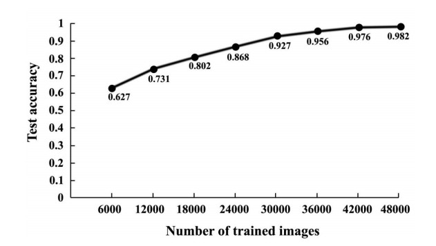
Patients with craniocerebral injury are in serious condition and inconvenient to take care of. This paper proposes a method of extracting the patient's body behavior feature based on convolution neural network, in order to reduce nursing workload and save hospital costs. The algorithm adopts double network model design, including the patient detection network model and the patient's body behavior feature extraction model. The algorithm is applied to the patient's body behavior detection system, so as to realize the recognition and monitoring of patients and improve the level of intelligent medical care for craniocerebral injury. Finally, the open source framework platform is used to test the patient behavior detection system. The experimental results show that the larger the test data set is, the higher the accuracy of patient body behavior feature extraction is. The average recognition rate of patient body behavior category is 97.8%, which verifies the effectiveness and correctness of the system. The application of convolution neural network connects image recognition with intelligent medical nursing, which provides reference and experience for intelligent medical nursing of patients with craniocerebral injury.

References

[1]	D. S. Burstein, Conflating medical care with patient care, J. Grad. Med. Educ., 9 (2017), 671. doi: 10.4300/JGME-D-17-00458.1
[2]	E. Codier, D. D. Codier, Could emotional intelligence make patients safer, Am. J. Nurs., 117 (2017), 58-62.
[3]	R. Diver, T. Quince, S. Barclay, J. Benson, J. Brimicombe, D. Wood, et al., Palliative care in medical practice: medical students' expectations, BMJ Support Palliat Care, 8 (2018), 285-288. doi: 10.1136/bmjspcare-2017-001486
[4]	S. M. Anwar, M. Majid, A. Qayyum, M. Awais, M. Alnowami, M. K. Khan, Medical image analysis using convolutional neural networks: a review, J. Med. Syst., 42 (2018), 226. doi: 10.1007/s10916-018-1001-y
[5]	W. Luo, W. Yang, Y. Zhang, Convolutional neural network for detecting odontocete echolocation clicks, J. Acoust. Soc. Am., 145 (2019), 7. doi: 10.1121/1.5085647
[6]	M. Galgano, G. Toshkezi, X. Qiu, T. Russell, L. Chin, L. R. Zhao, Traumatic brain injury: current treatment strategies and future endeavors, Cell Transplant, 26 (2017), 1118-1130. doi: 10.1177/0963689717714102
[7]	A. Khellaf, D. Z. Khan, A. Helmy, Recent advances in traumatic brain injury, J. Neur., 266 (2019), 2878-2889. doi: 10.1007/s00415-019-09541-4
[8]	D. Najem, K. Rennie, M. Ribecco-Lutkiewicz, D. Ly, J. Haukenfrers, Q. Liu, et al., Traumatic brain injury: classification, models, and markers, Biochem. Cell Biol., 96 (2018), 391-406. doi: 10.1139/bcb-2016-0160
[9]	W. Lina, J. Ding, Behavior detection method of openpose combined with Yolo network, (2020), 326-330.
[10]	S. Sivamani, S. H. Choi, D. H. Lee, J. Park, S. Chon, Automatic posture detection of pigs on real-time using Yolo framework, Int. J. Res. Trends Innov., 5 (2020), 81-88.
[11]	M. Sarıgül, B. M. Ozyildirim, M. Avci, Differential convolutional neural network, Neur. Netw., 116 (2019), 279-287. doi: 10.1016/j.neunet.2019.04.025
[12]	P. Xuan, S. Pan, T. Zhang, Y. Liu, H. Sun, Graph convolutional network and convolutional neural network based method for predicting lncRNA-disease associations, Cells, 8 (2019).
[13]	K. Yasaka, H. Akai, A. Kunimatsu, S. Kiryu, O. Abe, Deep learning with convolutional neural network in radiology, Jpn. J. Radiol., 36 (2018), 257-272. doi: 10.1007/s11604-018-0726-3
[14]	A. O. Alia, M. L. Petrunich-Rutherford, Anxiety-like behavior and whole-body cortisol responses to components of energy drinks in zebrafish (Danio rerio), Peer J., 7 (2019), e7546. doi: 10.7717/peerj.7546
[15]	F. Barthels, J. Kisser, R. Pietrowsky, Orthorexic eating behavior and body dissatisfaction in a sample of young females, Eat. Weight Disord., 2020.
[16]	A. Mathis, P. Mamidanna, K. M. Cury, T. Abe, V. N. Murthy, M. W. Mathis, et al., DeepLabCut: markerless pose estimation of user-defined body parts with deep learning, Nat. Neurosci., 21 (2018), 1281-1289. doi: 10.1038/s41593-018-0209-y
[17]	E. Štefanová, P. Bakalár, T. Baška, Eating-disordered behavior in adolescents: associations with body image, body composition and physical activity, Int. J. Environ. Res. Public Health, 17 (2020).
[18]	E. Yilmaz, Influence of lubricating conditions on the two-body wear behavior and hardness of titanium alloys for biomedical applications, Comput. Methods Biomech. Biomed. Engin., 23 (2020), 1377-1386. doi: 10.1080/10255842.2020.1804882
[19]	M. Atzori, H. Müller, PaWFE: Fast signal feature extraction using parallel time windows, Front. Neur., 13 (2019), 74. doi: 10.3389/fnins.2019.00074
[20]	X. Fang, N. Han, J. Wu, Y. Xu, J. Yang, W. K. Wong, et al., Approximate low-rank projection learning for feature extraction, IEEE Trans. Neur. Netw. Learn. Syst., 29 (2018), 5228-5241. doi: 10.1109/TNNLS.2018.2796133
[21]	Q. Shi, Y. M. Cheung, Q. Zhao, H. Lu, Feature extraction for incomplete data via low-rank tensor decomposition with feature regularization, IEEE Trans. Neur. Netw. Learn. Syst., 30 (2019), 1803-1817. doi: 10.1109/TNNLS.2018.2873655
[22]	Z. Y. Zhang, D. D. Gui, M. Sha, J. Liu, H. Y. Wang, Raman chemical feature extraction for quality control of dairy products, J. Dairy Sci., 102 (2019), 68-76. doi: 10.3168/jds.2018-14569

Reader Comments

Your name:*

Email:*
© 2021 the Author(s), licensee AIMS Press. This is an open access article distributed under the terms of the Creative Commons Attribution License (http://creativecommons.org/licenses/by/4.0)