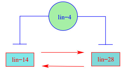
MicroRNAs are known to regulate gene expression either by repressing translation or by directing sequence-specific degradation of target mRNAs, and are therefore considered to be key regulators of gene expression. A gene-regulatory pathway involving heterochronic genes controls the temporal pattern of Caenorhabditis elegans postembryonic cell lineages. Based on experimental data, we propose and analyze a mathematical model of a gene-regulatory module in this nematode involving two heterochronic genes, lin-14 and lin-28, which are both regulated by lin-4, encoding a microRNA. The conditions under which the model experiences bifurcations are investigated. We determine the parameter regimes for which the system exhibits monostability and bistability, the latter associated with a biological switch. We observe in particular that bistability occurs without co-operativity, in keeping with knowledge about the regulatory behaviour of lin-14 and lin-28. The analytical results are confirmed by numerical simulations that illustrate how the microRNA lin-4 plays a crucial role in determining of the qualitative dynamics of the model.
Citation: Mainul Haque, John R. King, Simon Preston, Matthew Loose, David de Pomerai. Mathematical modelling of a microRNA-regulated gene network in Caenorhabditis elegans[J]. Mathematical Biosciences and Engineering, 2020, 17(4): 2881-2904. doi: 10.3934/mbe.2020162
MicroRNAs are known to regulate gene expression either by repressing translation or by directing sequence-specific degradation of target mRNAs, and are therefore considered to be key regulators of gene expression. A gene-regulatory pathway involving heterochronic genes controls the temporal pattern of Caenorhabditis elegans postembryonic cell lineages. Based on experimental data, we propose and analyze a mathematical model of a gene-regulatory module in this nematode involving two heterochronic genes, lin-14 and lin-28, which are both regulated by lin-4, encoding a microRNA. The conditions under which the model experiences bifurcations are investigated. We determine the parameter regimes for which the system exhibits monostability and bistability, the latter associated with a biological switch. We observe in particular that bistability occurs without co-operativity, in keeping with knowledge about the regulatory behaviour of lin-14 and lin-28. The analytical results are confirmed by numerical simulations that illustrate how the microRNA lin-4 plays a crucial role in determining of the qualitative dynamics of the model.

| [1] |
R. C. Lee, R. L. Feinbaum, V. Ambros, The C. elegans heterochronic gene lin-4 encodes small RNAs with antisense complimentarity to lin-14, Cell, 75 (1993), 843-843. doi: 10.1016/0092-8674(93)90529-Y

|
| [2] |
G. Ruvkun, Molecular biology: Glimpses of a tiny RNA world, Science, 294 (2001), 797-799. doi: 10.1126/science.1066315
|
| [3] |
A. M. Denli, B. B. J. Tops, R. H. A. Plasterk, R. F. Ketting, G. J. Hannon, Processing of primary microRNAs by the Microprocessor complex, Nature, 432 (2004), 231-235. doi: 10.1038/nature03049
|
| [4] |
G. Meister, M. Landthaler, Y. Dorsett, T. Tuschl, Sequence-specific inhibition of microRNA-and siRNA-induced RNA silencing, RNA, 10 (2004), 544-550. doi: 10.1261/rna.5235104
|
| [5] |
R. F. Place, L. Li, D. Pookot, E. J. Noonan, R. Dahiya, MicroRNA-373 induces expression of genes with complementary promoter sequences, Proc. Natl. Acad. Sci. USA, 105 (2008), 1608-1613. doi: 10.1073/pnas.0707594105
|
| [6] |
J. C. Carrington, V. Ambros, Role of microRNAs in plant and animal development, Science, 301 (2003), 336-338. doi: 10.1126/science.1085242
|
| [7] |
J. Lu, G. Getz, E. A. Miska, E. Alvarez-Saavedra, J. Lamb, D. Peck, et al., MicroRNA expression profiles classify human cancers, Nature, 435 (2005), 834-838. doi: 10.1038/nature03702
|
| [8] | H. Hwang, J. T. Mendell, MicroRNAs in cell proliferation, cell death, and tumorigenesis, Br. J. Cancer, 94 (2006), 776-780. |
| [9] |
G. Martello, L. Zacchigna, M. Inui, M. Montagner, M. Adorno, A. Mamidi, et al., MicroRNA control of Nodal signalling, Nature, 449 (2007), 183-188. doi: 10.1038/nature06100
|
| [10] |
M. Kato, T. Paranjape, R. Ullrich, S. Nallur, E. Gillespie, K. Keane, et al., The mir-34 microRNA is required for the DNA damage response in vivo in C. elegans and in vitro in human breast cancer cells, Oncogene, 28 (2009), 2419-2424. doi: 10.1038/onc.2009.106
|
| [11] |
G. T. Bommer, I. Gerin, Y. Feng, A. J. Kaczorowski, R. Kuick, R. E. Love, et al., p53-mediated activation of mirna34 candidate tumor-suppressor genes, Curr. Biol., 17 (2007), 1298-1307. doi: 10.1016/j.cub.2007.06.068
|
| [12] |
T. Chang, E. A. Wentzel, O. A. Kent, K. Ramachandran, M. Mullendore, K. H. Lee, et al., Transactivation of mir-34a by p53 broadlyáinfluences gene expression andpromotesapoptosis, Mol. Cell, 26 (2007), 745-752. doi: 10.1016/j.molcel.2007.05.010
|
| [13] |
L. He, X. He, L. P. Lim, E. De Stanchina, Z. Xuan, Y. Liang, et al., A microrna component of the p53 tumour suppressor network, Nature, 447 (2007), 1130-1134. doi: 10.1038/nature05939
|
| [14] |
H. Liu, X. Tian, Y. Li, C. Wu, C. Zheng, Microarray-based analysis of stress-regulated microRNAs in Arabidopsis thaliana, RNA, 14 (2008), 836-843. doi: 10.1261/rna.895308
|
| [15] |
R. Feinbaum, V. Ambros, The timing of lin-4RNA accumulation controls the timing of postembryonic developmental events in Caenorhabditis elegans, Dev. Biol., 210 (1999), 87-95. doi: 10.1006/dbio.1999.9272
|
| [16] |
V. R. Ambros H. R. Horvitz, The lin-14 locus of Caenorhabditis elegans controls the time of expression of specific postembryonic developmental events, Genes Dev., 1 (1987), 398-414. doi: 10.1101/gad.1.4.398
|
| [17] |
V. Ambros, A hierarchy of regulatory genes controls a larva-to-adult developmental switch in C. elegans, Cell, 57 (1989), 49-57. doi: 10.1016/0092-8674(89)90171-2
|
| [18] | M. Haque, Mathematical Modelling of Eukaryotic Stress-Response Gene Networks, PhD thesis, University of Nottingham, 2012. |
| [19] |
K. Seggerson, L. Tang, E. G. Moss, Two genetic circuits repress the Caenorhabditis elegans heterochronic gene lin-28 after translation initiation, Dev. Biol., 243 (2002), 215-225. doi: 10.1006/dbio.2001.0563
|
| [20] |
P. Arasu, B. Wightman, G. Ruvkun, Temporal regulation of lin-14 by the antagonistic action of two other heterochronic genes, lin-4 and lin-28, Genes Dev., 5 (1991), 1825-1833. doi: 10.1101/gad.5.10.1825
|
| [21] |
M. Lagos-Quintana, R. Rauhut, W. Lendeckel, T. Tuschl, Identification of novel genes coding for small expressed RNAs, Science, 294 (2001), 853-858. doi: 10.1126/science.1064921
|
| [22] |
N. C. Lau, L. P. Lim, E. G. Weinstein, D. P. Bartel, An abundant class of tiny RNAs with probable regulatory roles in Caenorhabditis elegans, Science, 294 (2001), 858-862. doi: 10.1126/science.1065062
|
| [23] | U. Alon, An Introduction to Systems Biology: Design Principles of Biological Circuits, Chapman and Hall/CRC, 2007. |
| [24] | J. Sotomayor, Generic bifurcations of dynamical systems, in Dynamical Systems, Academic Press, (1973), 561-582. |
| [25] |
E. G. Moss, R. C. Lee, V. Ambros, The cold shock domain protein lin-28 controls developmental timing in C. elegans and is regulated by the lin-4 RNA, Cell, 88 (1997), 637-646. doi: 10.1016/S0092-8674(00)81906-6
|
| [26] |
J. L. Cherry, F. R. Adler, How to make a biological switch, J. Theor. Biol., 203 (2000), 117-133. doi: 10.1006/jtbi.2000.1068
|
| [27] |
M. C. Ow, N. J. Martinez, P. H. Olsen, H. S. Silverman, M. I. Barrasa, B. Conradt, et al., The FLYWCH transcription factors FLH-1, FLH-2, and FLH-3 repress embryonic expression of microRNA genes in C. elegans, Genes Dev., 22 (2008), 2520-2534. doi: 10.1101/gad.1678808
|
| [28] | W. Rudin, Principles of Mathematical Analysis, 3rd edition, McGraw-Hill, New York, 1976. |
Figures(8) / Tables(4)

Mainul Haque, John R. King, Simon Preston, Matthew Loose, David de Pomerai. Mathematical modelling of a microRNA-regulated gene network in Caenorhabditis elegans[J]. Mathematical Biosciences and Engineering, 2020, 17(4): 2881-2904. doi: 10.3934/mbe.2020162


 DownLoad: