A novel distance of intuitionistic trapezoidal fuzzy numbers and its-based prospect theory algorithm in multi-attribute decision making model

Haiping Ren; Laijun Luo; Haiping Ren; Laijun Luo

doi:10.3934/mbe.2020163

Mathematical Biosciences and Engineering

2020, Volume 17, Issue 4: 2905-2922. doi: 10.3934/mbe.2020163

Previous Article Next Article

Research article Special Issues

A novel distance of intuitionistic trapezoidal fuzzy numbers and its-based prospect theory algorithm in multi-attribute decision making model

Haiping Ren ^{1
,
,},
Laijun Luo ²

1.
Teaching Department of Basic Subjects, Jiangxi University of Science and Technology, Nanchang, 330013, China
2.
School of Software and Engineering, Jiangxi University of Science and Technology, Nanchang, 330013, China

Received: 30 December 2019 Accepted: 17 March 2020 Published: 30 March 2020

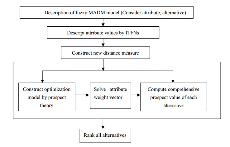
The aim of this paper is to develop a new decision making method considering decision makers' psychological behavior for multi-attribute decision making problem under intuitionistic trapezoidal fuzzy environment. We first put forward a new distance measure of intuitionistic trapezoidal fuzzy numbers. Then combining with cumulative prospect theory, we develop a novel decision making method, which can consider risk attitude of decision makers. Finally, an example is given to demonstrate the effectiveness and practicability of the proposed method.
- intuitionistic trapezoidal fuzzy number,
- distance measure,
- multi-attribute decision making method,
- prospect theory,
- risk attitude
Citation: Haiping Ren, Laijun Luo. A novel distance of intuitionistic trapezoidal fuzzy numbers and its-based prospect theory algorithm in multi-attribute decision making model[J]. Mathematical Biosciences and Engineering, 2020, 17(4): 2905-2922. doi: 10.3934/mbe.2020163

Related Papers:

Abstract

The aim of this paper is to develop a new decision making method considering decision makers' psychological behavior for multi-attribute decision making problem under intuitionistic trapezoidal fuzzy environment. We first put forward a new distance measure of intuitionistic trapezoidal fuzzy numbers. Then combining with cumulative prospect theory, we develop a novel decision making method, which can consider risk attitude of decision makers. Finally, an example is given to demonstrate the effectiveness and practicability of the proposed method.

References

[1]	G. Kou, P. Yang, Y. Peng, F. Xiao, Y. Chen, F. E. Alsaadic, Evaluation of feature selection methods for text classification with small datasets using multiple criteria decision-making methods, Appl. Soft Comput., 86 (2020), 105836. doi: 10.1016/j.asoc.2019.105836
[2]	G. Kou, D. Ergu, C. S. Lin, Y. Chen, Pairwise comparison matrix in multiple criteria decision making, Technol. Econ. Dev. Econ., 22 (2016), 738-765. doi: 10.3846/20294913.2016.1210694
[3]	G. Kou, Y. Q. Lu, Y. Peng, Y. Shi, Evaluation of classification algorithms using MCDM and rank correlation, Int. J. Inf. Tech. Decis., 11 (2012), 197-225. doi: 10.1142/S0219622012500095
[4]	R. Joshi, S. Kumar, An exponential Jensen fuzzy divergence measure with applications in multiple attribute decision-making, Math. Probl. Eng., 2018 (2018), 4342098.
[5]	G. Kou, Y. Peng, G. X. Wang, Evaluation of clustering algorithms for financial risk analysis using MCDM methods, Inform. Sciences, 275 (2014), 1-12 doi: 10.1016/j.ins.2014.02.137
[6]	H. Garg, K. Kumar, Distance measures for connection number sets based on set pair analysis and its applications to decision-making process, Appl. Intell., 48 (2018), 3346-3359. doi: 10.1007/s10489-018-1152-z
[7]	L. A. Zadeh, Fuzzy Sets, Inform. Control, 8 (1965), 338-353. doi: 10.1016/S0019-9958(65)90241-X
[8]	T. Jie, F. Meng, A consistency-based method to decision making with triangular fuzzy multiplicative preference relations, Int. J. Fuzzy Syst., 19 (2017), 1317-1332. doi: 10.1007/s40815-017-0333-y
[9]	A. Ebrahimnejad, J. L. Verdegay, H. Garg, Signed distance ranking based approach for solving bounded interval-valued fuzzy numbers linear programming problems, Int. J. Intell. Syst., 34 (2019), 2055-2076. doi: 10.1002/int.22130
[10]	K. T. Atanassov, Intuitionistic fuzzy sets, Fuzzy Set. Syst., 20 (1986), 87-96. doi: 10.1016/S0165-0114(86)80034-3
[11]	K. T. Atanassov, G. Gargov, Interval valued intuitionistic fuzzy sets, Fuzzy Set. Syst., 31 (1989), 343-349. doi: 10.1016/0165-0114(89)90205-4
[12]	H. Garg, An improved cosine similarity measures for intuitionistic fuzzy sets and their applications to decision-making process, Hacet. J. Math. Stat., 47 (2018), 1585-1601.
[13]	M. I. Ali, F. Feng, T. Mahmood, I. Mahmood, H. Faizan, A graphical method for ranking Atanassov's intuitionistic fuzzy values using the uncertainty index and entropy, Int. J. Intell. Syst., 34 (2019), 2692-2712. doi: 10.1002/int.22174
[14]	F. Feng, M. Liang, H. Fujita, R. R.Yager, X. Y. Liu, Lexicographic orders of intuitionistic fuzzy values and their relationships, Mathematics, 7 (2019), 166. doi: 10.3390/math7020166
[15]	P. Liu, Multiple attribute group decision making method based on interval-valued intuitionistic fuzzy power heronian aggregation operators, Comput. Ind. Eng., 108 (2017), 199-212. doi: 10.1016/j.cie.2017.04.033
[16]	H. Garg, K. Kumar, A novel exponential distance and its based TOPSIS method for interval-valued intuitionistic fuzzy sets using connection number of SPA theory, Artif. Intell. Rev., 53 (2020), 595-624. doi: 10.1007/s10462-018-9668-5
[17]	H. Garg, K. Kumar, Novel distance measures for cubic intuitionistic fuzzy sets and their applications to pattern recognitions and medical diagnosis, Granul. Comput., 5 (2020), 169-184. doi: 10.1007/s41066-018-0140-3
[18]	A. Si, S. Das, S. Kar, An approach to rank picture fuzzy numbers for decision making problems, Decis. Ma-Appl. Manage. Eng., 2 (2019), 54-64.
[19]	F. Liu, A. W. Guan, V. Lukovac, M. Vukić, A multicriteria model for the selection of the transport service provider: A single valued neutrosophic DEMATEL multicriteria model, Decis. Ma-Appl. Manage. Eng., 1 (2018), 121-130. doi: 10.31181/dmame1801121r
[20]	J. H. Hu, L. Pan, Y. Yang, H. W. Chen, A group medical diagnosis model based on intuitionistic fuzzy soft sets, Appl. Soft Comput., 77 (2019), 453-466. doi: 10.1016/j.asoc.2019.01.041
[21]	F. Feng, H. Fujita, M. I. Ali, R. R. Yager, X. Liu, Another view on generalized intuitionistic fuzzy soft sets and related multiattribute decision making methods, IEEE T. Fuzzy Syst., 27 (2018), 474-488.
[22]	H. Garg, R. Arora, Generalized and group-based generalized intuitionistic fuzzy soft sets with applications in decision-making, Appl. Intell., 48 (2018), 343-356. doi: 10.1007/s10489-017-0981-5
[23]	T. M. Athira, J. Sunil, H. Garg, Entropy and distance measures of Pythagorean fuzzy soft sets and their applications, J. Intell. Fuzzy Syst., 37 (2019), 4071-4084. doi: 10.3233/JIFS-190217
[24]	P. D. Liu, H. Gao, J. H. Ma, Novel green supplier selection method by combining quality function deployment with partitioned Bonferroni mean operator in interval type-2 fuzzy environment, Inform. Sciences, 490 (2019), 292-316. doi: 10.1016/j.ins.2019.03.079
[25]	P. D. Liu, P. Wang, Multiple-attribute decision-making based on archimedean Bonferroni operators of q-rung orthopair fuzzy numbers, IEEE T. Fuzzy Syst., 27 (2019), 834-848. doi: 10.1109/TFUZZ.2018.2826452
[26]	P. D. Liu, S. Y. Ma, P. Wang, Multiple-attribute group decision-making based on q-rung orthopair fuzzy power Maclaurin symmetric mean operators, IEEE Trans. Syst. Man Cybern. Syst., 2018 (2018).
[27]	M. H. Shu, C. H. Cheng, J. R. Chang, Using intuitionistic fuzzy sets for fault-tree analysis on printed circuit board assembly, Microelectron. Reliab., 46 (2006), 2139-2148. doi: 10.1016/j.microrel.2006.01.007
[28]	J. Q. Wang, Z. Zhang, Programming method of multicriteria decision making based on intuitionistic fuzzy number with incomplete certain information, Control Decis., 23 (2008), 1145-1152.
[29]	J. Q. Wang, Z. Zhang, Aggregation operators on intuitionistic trapezoidal fuzzy number and its application to multi-criteria decision making problems, J. Syst. Eng. Electron., 20 (2009), 321-326.
[30]	J. Ye, Expected value method for intuitionistic trapezoidal fuzzy multicriteria decision-making problems, Expert Syst. Appl., 38 (2011), 11730-11734. doi: 10.1016/j.eswa.2011.03.059
[31]	J. Yuan, C. Li, A new method for multi-attribute decision making with intuitionistic trapezoidal fuzzy random variable, Int. J. Fuzzy Syst., 19 (2017), 15-26. doi: 10.1007/s40815-016-0184-y
[32]	D. Kahneman, A. Tversky, Prospect theory: an analysis of decision under risk, Econometrica, 47 (1979), 263-292. doi: 10.2307/1914185
[33]	P. D. Liu, Y. Li, An extended MULTIMOORA method for probabilistic linguistic multi-criteria group decision-making based on prospect theory, Comput. Ind. Eng., 136 (2019), 528-545. doi: 10.1016/j.cie.2019.07.052
[34]	A. Tversky, D. Kahneman, Advances in prospect theory: cumulative representation of uncertainty, J. Risk Uncertainty, 5 (1992), 297-323. doi: 10.1007/BF00122574
[35]	Z. S. Chen, S. H. Xiong, Y. L. Li, G. S. Qian, Approach for intuitionistic trapezoidal fuzzy random prospect decision making based on the combination of parameter estimation and score functions, J. Syst. Eng. Electron., 37 (2015), 851-862.
[36]	Q. G. Ma, Hesitant fuzzy multi-attribute group decision-making method based on prospect theory, Comput. Eng. Appl., 51 (2015), 249-253.
[37]	S. Z. Zeng, W. H. Su, J. Chen, Fuzzy decision making with induced heavy aggregation operators and distance measures, J. Intell. Fuzzy Syst., 26 (2014), 127-135. doi: 10.3233/IFS-120720
[38]	P. Grzegorzewski, Metrics and orders in space of fuzzy numbers, Fuzzy Set. Syst., 97 (1998), 83-94 doi: 10.1016/S0165-0114(96)00322-3
[39]	A. I. Ban, L. Coroianu, Nearest interval, triangular and trapezoidal approximation of a fuzzy number preserving ambiguity, Int. J. Approx. Reason., 53 (2012), 805-836 doi: 10.1016/j.ijar.2012.02.001
[40]	U. Sharma, S. Aggarwal, Solving fully fuzzy multi-objective linear programming problem using nearest interval approximation of fuzzy number and interval programming, Int. J. Fuzzy Syst., 20 (2018), 488-499. doi: 10.1007/s40815-017-0336-8
[41]	R. Joshi, S. Kumar, Jensen-Tsalli's intuitionistic fuzzy divergence measure and its applications in medical analysis and pattern recognition, Int. J. Uncertain. Fuzz., 27 (2019), 145-169. doi: 10.1142/S0218488519500077

Reader Comments

Your name:*

Email:*
© 2020 the Author(s), licensee AIMS Press. This is an open access article distributed under the terms of the Creative Commons Attribution License (http://creativecommons.org/licenses/by/4.0)