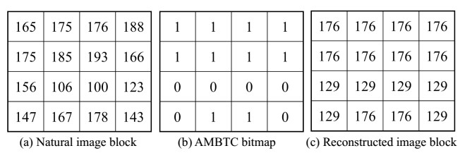
Citation: Cheonshik Kim, Dongkyoo Shin, Ching-Nung Yang. High capacity data hiding with absolute moment block truncation coding image based on interpolation[J]. Mathematical Biosciences and Engineering, 2020, 17(1): 160-178. doi: 10.3934/mbe.2020009
[1] | Yanlin Li, Mehraj Ahmad Lone, Umair Ali Wani . Biharmonic submanifolds of Kaehler product manifolds. AIMS Mathematics, 2021, 6(9): 9309-9321. doi: 10.3934/math.2021541 |
[2] | Fatemah Mofarreh, S. K. Srivastava, Anuj Kumar, Akram Ali . Geometric inequalities of PR-warped product submanifold in para-Kenmotsu manifold. AIMS Mathematics, 2022, 7(10): 19481-19509. doi: 10.3934/math.20221069 |
[3] | Yanyu Xiang, Aiping Wang . On symmetry of the product of two higher-order quasi-differential operators. AIMS Mathematics, 2023, 8(4): 9483-9505. doi: 10.3934/math.2023478 |
[4] | Mehmet Atçeken, Tuğba Mert . Characterizations for totally geodesic submanifolds of a K-paracontact manifold. AIMS Mathematics, 2021, 6(7): 7320-7332. doi: 10.3934/math.2021430 |
[5] | Fatimah Alghamdi, Fatemah Mofarreh, Akram Ali, Mohamed Lemine Bouleryah . Some rigidity theorems for totally real submanifolds in complex space forms. AIMS Mathematics, 2025, 10(4): 8191-8202. doi: 10.3934/math.2025376 |
[6] | Aliya Naaz Siddiqui, Meraj Ali Khan, Amira Ishan . Contact CR δ-invariant: an optimal estimate for Sasakian statistical manifolds. AIMS Mathematics, 2024, 9(10): 29220-29234. doi: 10.3934/math.20241416 |
[7] | Javier de Lucas, Julia Lange, Xavier Rivas . A symplectic approach to Schrödinger equations in the infinite-dimensional unbounded setting. AIMS Mathematics, 2024, 9(10): 27998-28043. doi: 10.3934/math.20241359 |
[8] | Tanumoy Pal, Ibrahim Al-Dayel, Meraj Ali Khan, Biswabismita Bag, Shyamal Kumar Hui, Foued Aloui . Generalized warped product submanifolds of Lorentzian concircular structure manifolds. AIMS Mathematics, 2024, 9(7): 17997-18012. doi: 10.3934/math.2024877 |
[9] | Hai-yan Zhang, Ji-jun Ao, Fang-zhen Bo . Eigenvalues of fourth-order boundary value problems with distributional potentials. AIMS Mathematics, 2022, 7(5): 7294-7317. doi: 10.3934/math.2022407 |
[10] | Mukhamed Aleroev, Hedi Aleroeva, Temirkhan Aleroev . Proof of the completeness of the system of eigenfunctions for one boundary-value problem for the fractional differential equation. AIMS Mathematics, 2019, 4(3): 714-720. doi: 10.3934/math.2019.3.714 |
Totally real submanifolds are one of the typical classes of submanifolds of Kaehler manifold. In 1974, B. Y. Chen and K. Ogiue [10] started the study of the totally real submanifolds from the point of view of their curvatures. Due to its geometrical importance, many geometers studied totally real submanifolds from the different point of views and various results were obtained in different ambient spaces [6,9,13,18]. Kaehler product manifold also attracts the attention of geometers toward itself [24]. S. Y. Cheng and S. T. Yau [11] obtained many well-known results introducing a self-adjoint differential operator ◻ defined by
◻f=n∑i,j=1(nHδij−ζn+1ij)fij, | (1.1) |
where f∈C2(N),(fij) is Hessian of f, H mean curvature, and ζn+1ij is the coefficients of second fundamental form ζ.
Using this differential operator H. Li [15] obtained a rigidity result for hypersurfaces in space forms with constant scalar curvature. In 2013, X. Gua and H. Li [17] extended the use of the operator for submanifolds and obtained interesting results for submanifolds with constant scalar curvature in a unit sphere.
Motivated by X. Gua and H. Li, we study the totally real submanifolds of Kaehler product manifold with constant scalar curvature using self-adjoint differential operator ◻ and obtain a characterization result.
Further, we study δ−invariant totally real submanifolds in same setting and prove some results.
Let (¯Nm,Jm,gm) and (¯Np,Jp,gp) are Kaehler manifolds of complex dimension m and complex dimension p respectively. Let Jm and gm be almost complex structure and metric tensor on ¯Nm respectively and Jp and gp almost complex structure and metric tensor on ¯Np respectively. Further, let us assume ¯Nm(c1) and ¯Np(c2) are complex space forms with constant holomorphic sectional curvatures c1 and c2 respectively.
We suppose ¯N(c1,c2)=¯Nm(c1)ׯNp(c2) the Kaehlerian product manifold with complex dimension (m+p). Let us denote by P and Q the projection operators of the tangent space of ¯N(c1,c2) to the tangent spaces of ¯Nm(c1) and ¯Np(c2) respectively. Then,
P2=P,Q2=Q,PQ=QP=0. |
By setting ϝ=P−Q, it can be easily shown that ϝ2=I. Thus, ϝ is an almost product structure on ¯N(c1,c2). Moreover, for a Riemannian metric g on ¯N(c1,c2) we have [20]
g(E,F)=gm(PE,PF)+gp(QE,QF), |
for all vector fields E,F on ¯N(c1,c2). We also have
g(ϝE,F)=g(ϝF,E). |
If we assume JE=JmPE+JpQE for any vector field E of ¯N(c1,c2). Then from [20], we see that
JmP=PJ,JpQ=QJ,ϝJ=Jϝ,J2=−I,g(JE,JF)=g(E,F),¯∇EJ=0. |
Therefore, J is a Kaehlerian structure on ¯N(c1,c2). Let ¯R be the Riemannian curvature tensor of a Kaehler product manifold ¯N(c1,c2). Then [24]
¯R(E,F,G,W)=116(c1+c2)[g(F,G)g(E,W)−g(E,G)g(F,W)+g(JF,G)g(JE,W)−g(JE,G)g(JF,W)+2g(JE,F)g(JG,W)+2g(ϝF,G)g(ϝE,W)−g(ϝE,G)g(ϝF,W)+g(ϝJF,G)g(ϝJE,W)−g(ϝJE,G)g(ϝJF,W)+2g(ϝE,JF)g(ϝJG,W)]+116(c1−c2)[g(ϝF,G)g(E,W)−g(ϝE,G)g(F,W)+g(F,G)g(ϝE,W)−g(E,G)g(ϝF,W)+g(ϝJF,G)g(JE,W)−g(ϝJE,G)g(JF,W)+g(JF,G)g(ϝJE,W)−g(JE,G)g(ϝJF,W)+2g(ϝE,JF)g(JG,W)+2g(E,JF)g(ϝJG,W)], | (2.1) |
for any vector fields E,F and G on ¯N(c1,c2).
Definition 2.1. Let N be a real n−dimensional Riemannian manifold isometrically immersed in a (m+p)− dimensional Kaehlerian product manifold ¯N(c1,c2). Then N is said to be totally real submanifold of ¯N(c1,c2) if JTx(N)⊥Tx(N) for each x∈N where Tx(N) denotes the tangent space to N at x∈N.
Let g be the metric tensor field on ¯N(c1,c2) as well as that induced on N. Also, we denote by ¯∇(resp. ∇) the Levi-Civita connection on ¯N(c1,c2)(resp. N). Then the Gauss and Weingarten formulas are given by
¯∇EF=∇EF+ζ(E,F), | (2.2) |
¯∇EN=−ΛNE+∇⊥EN, | (2.3) |
for all E,F tangent to N and vector field N normal to N, where ζ,∇⊥E and ΛN denote the second fundamental form, normal connection and shape operator respectively. The relation between the second fundamental form and the shape operator is given by
g(ζ(E,F),N)=g(ΛNE,F). | (2.4) |
We choose a local field of orthonormal frames e1,…,en;en+1,…,em+p;e1⋆=Je1,…,en⋆=Jen;e(n+1)⋆=Jen+1;e(m+p)⋆=Jem+p in ¯N(c1,c2) in such a way that restricted to N, the vectors e1,…,en are tangent to N. With respect to this frame field of ¯N(c1,c2), let ω1,…,ωn;ωn+1,…,ωm+p;ω1⋆,…,ωn⋆;ω(n+1)⋆,…,ω(m+p)⋆ be the field of dual frames. Unless otherwise stated, we use the following conventions over the range of indices:
A,B,C,D=1,…,m+p,1⋆,…,(m+p)⋆;i,j,k,l,t,s=1,…,n;α,β,γ=n+1,…,m+p;1⋆,…,(m+p)⋆;λ,μ,ν=n+1,…,m+p. |
Then the mean curvature vector H is defined as
H=∑αHαeα,whereHα=1n∑iζαii. | (2.5) |
Also, the structure equations of ¯N(c1,c2) are given by [24]
{dωA=−ωABωB,ωAB+ωBA=0,ωij+ωji=0,ωij=ωi⋆j⋆,ωi⋆j=ωj⋆i,ωλμ+ωμλ=0,ωλμ=ωλ⋆μ⋆,ωλ⋆μ=ωμ⋆λ. | (2.6) |
{ωiλ+ωλi=0,ωiμ=ωi⋆μ⋆,ωi⋆λ=ωλ⋆i,dωAB=−ωACωCB+ϕAB,ϕAB=12¯RABCDωC∧ωD. | (2.7) |
Restricting these forms to N, we have
ωα=0, | (2.8) |
dωi=−ωik∧ωk, | (2.9) |
dωij=−ωik∧ωkj+Ωij,Ωij=12Rijklωk∧ωl. | (2.10) |
Since 0=dωα=−ωαi∧ωi, by Cartan's Lemma we get
ωαi=ζαijωj,ζαij=ζαji, | (2.11) |
dωαβ=−ωαγ∧ωγβ+Ωαβ,Ωαβ=12Rαβklωk∧ωl. | (2.12) |
From (2.6) and (2.11) we find
ζi⋆jk=ζj⋆ik=ζk⋆ij. | (2.13) |
The covariant derivative of ζαij is given by
ζαijk=dζαij−ζαilωlj−ζαljωli+ζβijωαβ. | (2.14) |
The Laplacian Δζαij of ζαij is defined as
Δζαij=∑kζαijkk, | (2.15) |
where we have put ζαijklωl=dζαijk−ζαljkωli−ζαilkωlj−ζβijkωαβ.
Now, from [17] we have a trace-free linear map Θα:TxN→TxN given by
g(ΘαE,F)=g(ΛαE,F)−Hα(E,F), |
where x∈N and the shape operator Λα of eα is given by
Λα(ei)=−∑jg(¯∇eieα,ej)ej=∑jζαijej, |
and Θ is a bilinear map Θ:TxN×TxN→T⊥xN defined by
Θ(E,F)=m+p∑α=n+1g(ΘαE,F)eα. | (2.16) |
Then we have |Θ|2=|Λ|2−nH2, where H2=∑α(Hα)2.
The Gauss equation is given by
Rijkl=¯Rijkl+∑α(ζαikζαjl−ζαilζαjk). | (2.17) |
From (2.1) and Gauss equation, we obtain
2τ−116(c1+c2)n(n+1)=n2H2−|Λ|2, | (2.18) |
where τ is scalar curvature.
The Codazzi and the Ricci equation are respectively
ζαij,k=ζαik,l, | (2.19) |
R⊥αβij=∑k(ζαikζβkj−ζαjkζβki). | (2.20) |
Then, by using Codazzi equation one can easily see that the operator ◻ is self-adjoint. That is
∫N◻fdv=0,f∈C2(N). | (2.21) |
Since we have constant scalar curvature, Eq (2.18) implies that
|∇Λ|2=n2|∇H2|. | (2.22) |
We can choose a unit normal vector field en+1 which is parallel to H. Hence we have [16]
Hn+1=H,Hα=0(n+2≤α≤m+p), | (2.23) |
Θn+1ij=ζn+1ij−Hδij,Θαij=ζαij,(n+2≤α≤m+p). | (2.24) |
Now, we quote the following lemmas for later use.
Lemma 2.2. [19] Let B:Rn→Rn be a symmetric linear map such that trB=0, then
−n−2√n(n−1)|B|3≤trB3≤n−2√n(n−1)|B|3, |
where |B|2=trB2, and the equality holds if and only if at least n−1 eigenvalues of B are equal.
Lemma 2.3. [21] Let C,B:Rn→Rn be a symmetric linear map such that [C,B]=0 and trC=trB=0, then
−n−2√n(n−1)|C|2|B|≤tr(C2B)≤n−2√n(n−1)|C|2|B|. |
Lemma 2.4. [14] Let B1,B2,…,Bm, be symmetric (n×n)−matrices.
Set Sαβ=tr(BαBβ),Sα=Sαα,S=∑αSα, then
∑α,β|BαBβ−BβBα|2+∑α,βS2αβ≤32(∑αSα)2. |
This section is devoted to the proof of main result.
Theorem 3.1. Let Nn be a totally real submanifold in Kaehlerian product manifold ¯N(c1,c2)=¯Nm1(c1)ׯNp2(c2), c1,c2>0, with constant scalar curvature. If trϝ vanishes, then N is totally geodesic.
For proving that result, we need to prove the following preliminary Lemmas. Since ϝ is symmetric and J is skew-symmetric, following result is obvious.
Lemma 3.2. Let N be a totally real submanifold in Kaehler product manifold
¯N(c1,c2)=¯Nm1(c1)ׯNp2(c2), then trϝJ=trJϝ=0.
Lemma 3.3. Let N be a totally real submanifold in Kaehler product manifold
¯N(c1,c2)=¯Nm1(c1)ׯNp2(c2), then
12Δ|Λ|2=|∇Λ|2+∑α,i,j,kζαijζαkkij+116(c1+c2)∑α[(n+9+6(trϝ)2)trΛ2α−(3+(trϝ)2)]+116(c1−c2)∑α[(n+1)(trϝ)trΛ2α−2(trϝ)(trΛα)2]+116(c1+c2)∑t[(4(trϝ)2−2)trΛ2t−(1+(trϝ)2)(trΛt)2]+116(c1−c2)∑t[2(trϝ)trΛ2t−2(trϝ)(trΛt)2]−∑α,β,i,j(R⊥αβij)2−∑α,β(ζαijζβkl)2+∑α,βnHβζβklζαjlζαjk. | (3.1) |
Proof. From [12], we have
∑α,i,jζαijΔζαij=∑α,i,j,k(ζαijζαkkij−¯Rαijβζαijζβkk+4¯Rαβkiζβjkζαjk−¯Rαkβkζαijζβij+2¯Rlkikζαljζαij+2¯Rlijkζαlkζαij)−∑α,β,i,j,k,l(ζαikζβjk−ζαjkζβik)(ζαilζβjl−ζαjlζβil)−∑α,β,i,j,k,lζαijζαklζβijζβkl+∑α,β,i,j,k,lζαjiζαkiζβkjζβll. | (3.2) |
On the other hand, one has
∑α,i,jζαijΔζαij=12Δ|Λ|2−|∇Λ|2. | (3.3) |
By using Eqs (2.5), (2.20) and (3.3) in (3.2), we obtain
12Δ|Λ|2=|∇Λ|2+∑α,i,j,kζαijζαkkij+∑α,i,j,k(−¯Rαijβζαijζβkk+4¯Rαβkiζβjkζαjk−¯Rαkβkζαijζβij+2¯Rlkikζαljζαij+2¯Rlijkζαlkζαij)−∑α,β,i,j(R⊥αβij)2−∑α,β(ζαijζβkl)2+∑α,βnHβζβkjζαjiζαki. | (3.4) |
Using (2.1) and Lemma 3.2, we now compute the values of curvature terms involving ¯R of the Eq (3.4) as follows:
¯Rαijβζαijζβkk=g(¯R(ej,eβ)ei,eα)ζαijζβkk=116(c1+c2)[∑αtrΛ2α−3∑t(trΛt)2−3∑t(trϝ)2(trΛt)2−∑α(trϝ)2(trΛα)2]+116(c1−c2)[−2(trϝ)∑α(trΛα)2−∑t6(trϝ)(trΛt)2]. | (3.5) |
Similarly we obtain,
¯Rαβkiζβjkζαij=g(¯R(ek,ei)eβ,eα)ζβjkζαij=116(c1+c2)[∑t(trΛ2t)−∑t(trΛt)2+∑α(trΛ2α)+∑t(trϝ)2(trΛ2t)−∑t(trϝ)2(trΛt)2]+116(c1−c2)[2∑t(trϝ)(trΛ2t)−2∑t(trϝ)(trΛt)2], | (3.6) |
¯Rαkβkζαijζβij=g(¯R(eβ,ek)ek,eα)ζαijζβij=116(c1+c2)[(n−1)∑α(trΛ2α)+∑t6(trΛ2t)+2∑α(trϝ)2(trΛ2α)]+116(c1−c2)[(n+1)∑α(trϝ)(trΛ2α)+∑t6(trϝ)(trΛ2t)], | (3.7) |
¯Rlkikζαljζαij=g(¯R(ei,ek)ek,el)ζαljζαij=116(c1+c2)[∑αn(trΛ2α)+∑α2(trϝ)(trΛ2α)+∑α(trΛ2α)]+116(c1−c2)[n∑α(trϝ)(trΛ2α)−∑α(trϝ)(trΛ2α)], | (3.8) |
and
¯Rlijkζαlkζαij=g(¯R(ej,ek)ei,el)ζαlkζαij=116(c1+c2)[∑α(trΛ2α)−∑α(trΛα)2+∑α(trϝ)2(trΛ2α)−∑α(trϝ)2(trΛα)2]+116(c1−c2)[2∑α(trϝ)(trΛ2α)−2∑α(trϝ)(trΛα)2]. | (3.9) |
Thus, making use of Eqs (3.5)–(3.9) in (3.4), we get (3.1).
Proof of Theorem 3.1. From (1.1) and (2.22), we obtain
◻(nH)=12Δ|Λ|2−n2|∇H|2−∑nζijH,ij. | (3.10) |
Now, using (3.1) in the above equation, we get
◻(nH)=|∇Λ|2+∑α,i,j,kζαijζαkkij+116(c1+c2)∑α[(n+9+6(trϝ)2)trΛ2α−(3+(trϝ)2)]+116(c1−c2)∑α[(n+1)(trϝ)trΛ2α−2(trϝ)(trΛα)2]+116(c1+c2)∑t[(4(trϝ)2−2)trΛ2t−(1+(trϝ)2)(trΛt)2]+116(c1−c2)∑t[2(trϝ)trΛ2t−2(trϝ)(trΛt)2]−∑α,β,i,j(R⊥αβij)2−∑α,β(ζαijζβkl)2+∑α,βnHβζβklζαjlζαjk−n2|∇H|2−∑nζijH,ij, |
which implies
◻(nH)=116(c1+c2)∑α[(n+9+6(trϝ)2)trΛ2α−(3+(trϝ)2)]+116(c1−c2)∑α[(n+1)(trϝ)trΛ2α−2(trϝ)(trΛα)2]+116(c1+c2)∑t[(4(trϝ)2−2)trΛ2t−(1+(trϝ)2)(trΛt)2]+116(c1−c2)∑t[2(trϝ)trΛ2t−2(trϝ)(trΛt)2]−∑α,β,i,j(R⊥αβij)2−∑α,β(ζαijζβkl)2+∑α,βnHβζβklζαjlζαjk. | (3.11) |
A direct computation gives
∑α(trΛα)2=∑αζαiiζαjj=n2H2. | (3.12) |
Moreover, it is easy to see that
∑α(trΛ2α)=∑αζαijζαij=|Θ|2+nH2 | (3.13) |
and
∑α(trΛ2t)=‖ζ⋆‖2, | (3.14) |
where ζ⋆ij=g(ζ(ei,ej),et⋆) and ζij=¯ζij⊕ζ⋆ij.
Also we have
∑α,β(ζαijζβkl)2+∑α,β,i,j(R⊥αβij)2=∑α,β[tr(ΛαΛβ)]2+∑α≠n+1,β≠n+1,i,j(R⊥αβij)2. | (3.15) |
Using Lemma 2.4 in (3.15), we get
∑α,β(ζαijζβkl)2+∑α,β,i,j(R⊥αβij)2≤[tr(Λn+1Λn+1)]2+2∑β≠n+1(trΛn+1Λβ)2+32[∑β≠n+1|Θβ|2]2=52|Θn+1|4+2nH2|Θn+1|2+n2H4+2∑β≠n+1(trΘn+1Θβ)2−2(trΘn+1Θn+1)2+32|Θ|4−3|Θ|2|Θn+1|2≤52|Θn+1|4+2nH2|Θn+1|2+n2H4+2|Θn+1|2(|Θ|2−|Θn+1|2)+32|Θ|4−3|Θ|2|Θn+1|2=12|Θn+1|4+2nH2|Θn+1|2+n2H4−|Θ|2|Θn+1|2+32|Θ|4. | (3.16) |
Taking into account the Eq (2.24), we derive
∑α,β,i,j,kHβζβklζαjlζαjk=∑α,i,j,kHζn+1klζαjlζαjk=Htr(Θn+1)3+3H2(Θn+1)2+nH4+3trΘn+1H2+m+p∑α=n+2H2|Θα|2+m+p∑α=n+2∑i,j,kHΘn+1ijΘαjkΘαki. | (3.17) |
Taking Lemma 2.2 and Eq (3.17) into account, we have
∑α,β,i,j,kHβζβklζαjlζαjk≥−n−2√n(n−1)|Θn+1|3|H|+3H2|Θn+1|2+nH4+(∑α=n+2H2|Θα|2−H2|Θn+1|2)+∑α=n+2Htr(Θn+1)(Θα)2. | (3.18) |
Which by virtue of Lemma 2.3 and (3.18), yields
∑α,β,i,j,kHβζβklζαjlζαjk≥−n−2√n(n−1)|Θn+1|3|H|+3H2|Θn+1|2+nH4+H2|Θ|2−n−2√n(n−1)∑α=n+2|Θn+1||Θα|2|H|=2H2|Θn+1|2+H2|Θ|2+nH4−n−2√n(n−1)|Θn+1||Θ|2|H|. | (3.19) |
Now, substituting (3.12)–(3.14), (3.16) and (3.19) in (3.11), we find
◻(nH)≥116(c1+c2)[(n+9+6(trϝ)2)(|Θ|2+nH2)−3−(trϝ)2]+116(c1−c2)[(trϝ)(n|Θ|2−n2H2+|Θ|2+nH2)]+116(c1+c2)[(4(trϝ)2−2)‖ζ⋆‖2]+116(c1−c2)[2(trϝ)‖ζ⋆‖2]−n−2√n(n−1)|Θn+1|Θ|2||H|+nH2|Θ|2−12|Θn+1|4+|Θ|2|Θn+1|2−32|Θ|4=116(c1+c2)[(n+9+6(trϝ)2)(|Θ|2+nH2)−3−(trϝ)2]+116(c1−c2)[(trϝ)(n|Θ|2−n2H2+|Θ|2+nH2)]+116(c1+c2)[(4(trϝ)2−2)‖ζ⋆‖2]+116(c1−c2)[2(trϝ)‖ζ⋆‖2]+|Θ|2[−n−2√n(n−1)|Θ||H|+nH2−|Θ|2]+(|Θ|−|Θn+1|)[n−2√n(n−1)|Θ|2|H|−12(|Θ|−|Θn+1|)(|Θ|+|Θn+1|)2]. | (3.20) |
It is known that [17],
(|Θ|−|Θn+1|)[n−2√n(n−1)|Θ|2|H|−12(|Θ|−|Θn+1|)(|Θ|+|Θn+1|)2]≥0. |
Therefore, from (3.20) we have
◻(nH)≥116(c1+c2)[(n+9+6(trϝ)2)(|Θ|2+nH2)−3−(trϝ)2]+116(c1−c2)[(trϝ)(n|Θ|2−n2H2+|Θ|2+nH2)]+116(c1+c2)[(4(trϝ)2−2)‖ζ⋆‖2]+116(c1−c2)[2(trϝ)‖ζ⋆‖2]+|Θ|2[−n−2√n(n−1)|Θ||H|+nH2−|Θ|2]. | (3.21) |
Since, c1,c2>0 and trϝ=0. Then the above inequality implies the following inequality
◻(nH)≥116(c1+c2)[(n+9)(|Θ|2+nH2)−3−2‖ζ⋆‖2]+|Θ|2[−n−2√n(n−1)|Θ||H|+nH2−|Θ|2]≥116(c1+c2)[(n+9)(|Θ|2+nH2)]+nH2|Θ|2. | (3.22) |
From (2.21) we have ∫N◻(nH)dv=0. Thus we have following two cases:
Case 1:
|Θ|2+nH2=0 and nH2|Θ|2=0 |
which yields Λ=0 and H=0. Thus, the submanifold is totally geodesic.
Case 2:
116(c1+c2)(n+9)(|Θ|2+nH2)=−nH2|Θ|2 |
which implies that Λ=0 and H=0. It is again totally geodesic.
Hence, we have our assertion.
Now, we give an example in the support of the Theorem 3.1.
Example. It is known that the real projective space RPn(1) is totally geodesic submanifold of the complex projective space CPn(4) [3]. Also from [23] we know that, if N1 is any submanifolds of Kaehler manifold M1 and N2 is any submanifold of Kaehler manifold M2, then the natural product N=N1×N2 is a submanifold of the Kaehler product manifold M=M1×M2. Hence, RPn(1)×RPn(1) is a submanifolds of the Kaehler product manifold CPn(4)×CPn(4), which satisfies all the hypothesis of the Theorem 3.1 and indeed totally geodesic.
Remark 3.4. In the above example, it can be noticed that trϝ vanishes, due to the fact that the projection operators P and Q coincide.
Let N be a Riemannian manifold and K(π) denotes the sectional curvature of N of the plane section π⊂TxN at a point x∈N. Let {e1,…,en} and {en+1,…,e2(m+p)} be the orthonormal basis of TxN and T⊥xN at any x∈N, then the scalar curvature τ at that point is given by
τ(x)=∑1≤i<j≤nK(ei∧ej). |
If we consider that L is an r-dimensional subspace of TN, r≥2, and {e1,e2,…,er} is an orthonormal basis of L. Then the scalar curvature of the r-plane section L is given as
τ(L)=∑1≤γ<β≤rK(eγ∧eβ),1≤γ,β≤r, | (4.1) |
for n≥3 and k≥1. Let us assume S(n,k) the finite set consisting of k−tuples (n1,…,nk) of integers satisfying
2≤n1,…,nk<nandn1+⋯+nk≤n. |
Also denote by S(n) the union ⋃k≥1S(n,k).
For each (n1,…,nk)∈S(n) and each point x∈N, B. Y. Chen [8] introduced a Riemannian invariant δ(n1,…,nk)(x) defined by
δ(n1,…,nk)(x)=τ(x)−inf{τ(L1)+⋯+τ(Lk)}, | (4.2) |
where L1,…,Lk run over all k mutually orthogonal subspaces of TxN such that dimLj=∑nj, j=1,…,k.
We recall the following Lemma [7]:
Lemma 4.1. Let a1,…,an,an+1 be n+1 real numbers such that
(n∑i=1ai)2=(n−1)(an+1+n∑i=1a2i). | (4.3) |
Then 2a1a2≥an+1, with equality holding if and only if a1+a2=a3=⋯=an.
In this section we state and prove the following.
Theorem 4.2. Let N be a totally real submanifold in Kaehler product manifold ¯N(c1,c2)=¯Nm1(c1)ׯNp2(c2) and if trP coincides with trQ, then
δ(n1,…,nk)≤n2(n+k−1−∑nj)2(n+k−∑nj)H2+132[n(n+1)−k∑j=1nj(nj+1)](c1+c2), | (4.4) |
and the equality holds in (4.4) if and only if at a point x∈N there exists an orthonormal basis e1,…,e2(m+p) at x such that the shape operator of N in ¯N(c1,c2) at x takes the forms:
Λr=(Λr1…0⋮ ⋱⋮O0…ΛrkOμrI), r=n+1,…,2(m+p), | (4.5) |
where O is a null matrix, I is an identity matrix and each Λrj is a symmetric nj×nj submatrix such that
tr(Λr1)=⋯=tr(Λrk)=μr. | (4.6) |
Proof. We put
ε=2τ−116(c1+c2)n(n+1)−n2(n+k−1−∑nj)2(n+k−∑nj)H2. | (4.7) |
By combining (2.18) and (4.7), we obtain
n2H2=(n+k−∑nj)(ε+|Λ|2). |
With respect to the orthonormal basis, the last equation can be written as
(n∑i=1ζn+1ii)2=(n+k−∑nj)(ε+n∑i=1(ζn+1ii)2+∑i≠j(ζn+1ij)2+2(m+p)∑r=n+2n∑i,j=1(ζrij)2), | (4.8) |
which implies that
(n∑i=1ai)2=(n+k−∑nj)(ε+n∑i=1(ai)2+∑i≠j(ζn+1ij)2+2(m+p)∑r=n+2n∑i,j=1(ζrij)2). | (4.9) |
Now, let us set
Δ1={1,…,n1},…,Δk={n1+⋯+nk−1+1,…,n1+⋯+nk}, |
and
¯a1=a1,¯a2=a2+⋯+an1,¯a3=an1+1+⋯+an1+n2,…,¯ak+1=an1+⋯+nk−1+1+⋯+an1+⋯+nk,¯ak+2=an1+⋯+nk+1,…,¯an+k+1−∑nj=an. |
Then Eq (4.9) is equivalent to
(n+k+1−∑nj∑i=1¯ai)2=(n+k−∑nj)(ε+n+k+1−∑nj∑i=1(¯ai)2+∑i≠j(ζn+1ij)2+2(m+p)∑r=n+2n∑i,j=1(ζrij)2)−∑2≤α1≠β1≤n1aα1aβ1−∑α1≠β1aα2aβ2−⋯−∑αk≠βkaαkaβk, | (4.10) |
where α2,β2∈Δ2,…,αk,βk∈Δk.
Using Lemma 4.1 in (4.10) yields
∑α1<β1aα1aβ1−∑α2<β2aα2aβ2−⋯−∑αk<βkaαkaβk≥ε2+∑i≠j(ζn+1ij)2+122(m+p)∑r=n+2n∑i,j=1(ζrij)2, | (4.11) |
where αj,βj∈Δj,j=1,…,k.
Furthermore, combining (4.1) with the Gauss equation, we obtain
τ(Lj)=132nj(nj+1)(c1+c2)+2(m+p)∑r=n+1∑αj<βj(ζrαjαjζrβjβj−(ζrαjβj)2). | (4.12) |
Combining (4.11) and (4.12) gives
τ(L1)+⋯+τ(Lk)≥ε2+132k∑j=1nj(nj+1)(c1+c2)+122(m+p)∑r=n+1∑(α,β)∉Δ2(ζrαβ)2+122(m+p)∑r=n+2k∑j=1(∑αj∈Δjζrαjαj)2≥ε2+132k∑j=1nj(nj+1)(c1+c2), | (4.13) |
where Δ=Δ1∪⋯∪Δk,Δ2=(Δ1×Δ1)∪⋯∪(Δk×Δk).
Thus, Eqs (4.2), (4.7) and (4.13) imply (4.4).
Moreover, equality in (4.11) and (4.13) holds at a point x, if it holds for (4.4) at a point x. In this case from Lemma 4.1 and Eqs (4.10)–(4.13), we have (4.5) and (4.6). A straightforward computation yields the converse part.
Example. Due to the fact that the real hyperbolic space Hn(1) can be isometrically embedded in the complex hyperbolic space CHn(−4) as a totally real totally geodesic submanifold of minimal codimension [22]. It follows that N=RPn(1)×RPn(1) is a totally real submanifold of M=HPn(4)×HPn(4). This submanifold satisfies all hypotheses of Theorem 4.2. In this case the inequality is satisfied with equality at all points.
Theorem 4.2 yields the following obstruction result.
Corollary 4.3. Let N be a totally real submanifold in Kaehler product manifold ¯N(c1,c2)=¯Nn1(c1)ׯNp2(c2) and if trϝ vanishes, then for c1+c2=0, N can not be minimally immersed in ¯N(c1,c2).
We characterized totally real submanifold using self-adjoint differential operator. The self-adjoint differential operators are mainly used in functional analysis and quantum mechanics. In quantum mechanics their importance lies in the Drac-Von Neumann formulation of quantum mechanics in which momentum, angular momentum and spin are represented by self-adjoint operators on Hilbert space. A self-adjoint differential operator is an important class of unbounded operators. Therefore, we can use such operator for infinite dimensional cases and we resemble the finite dimensional case. Thus, use of the operator for such characterization may open a new path to link results in differential geometry with quantum mechanics as well as well with functional analysis.
This work is supported by Taif University Researchers Supporting Project number (TURSP-2020/223), Taif University, Taif, Saudi Arabia.
The authors declare that there is no conflict of interests.
[1] | W. Bender, D. Gruhl, N. Morimoto, et al., Techniques for data hiding, IBM Syst. J., 35 (1996), 313-336. |
[2] | C. N. Yang, S. C. Hsu and C. Kim, Improving stego image quality in image interpolation based data hiding, Comput. Stand. Interfaces, 50 (2017), 209-215. |
[3] | C. Kim, D. Shin, C. N. Yang, et al., Improving capacity of Hamming (n,k)+1 stego-code by using optimized Hamming+k, Digital Signal Process., 78 (2018), 284-293. |
[4] | Y. Q. Shi, X. Li, X. Zhang, et al., Reversible data hiding: Advances in the past two decades, IEEE Access, 4 (2016), 3210-3237. |
[5] | F. Huang, X. Qu, H. J. Kim, et al., Reversible Data Hiding in JPEG Images, IEEE Trans. Circuits Syst. Video Technol., 26 (2016), 1610-1621. |
[6] | J. Mielikainen, LSB matching revisited, IEEE Signal Proc. Let., 13 (2006), 285-287. |
[7] | C. K. Chan and L. M. Cheng, Hiding data in images by simple LSB substitution, Pattern Recognit., 37 (2004), 469-474. |
[8] | C. C. Chang, C. C. Lin, C. S. Tseng, et al., Reversible hiding in DCT-based compressed images, Inf. Sci., 177 (2007), 2768-2786. |
[9] | C. C. Chang, T. S. Chen and L. Z. Chung, A steganographic method based upon JPEG and quantization table modification, Inf. Sci., 141 (2002), 123-138. |
[10] | C. Bergman and J. Davidson, Unitary embedding for data hiding with the SVD, Proceedings Volume 5681, Security, Steganography, and Watermarking of Multimedia Contents VⅡ, (2005). Available from: https://doi.org/10.1117/12.587796. |
[11] | E. Delp and O. Mitchell, Image compression using block truncation coding, IEEE Trans. Commun., 27 (1979), 1335-1342. |
[12] |
W. Hong, T. S. Chen and C. W. Shiu, Lossless steganography for AMBTC compressed images, 2008 Congress on Image and Signal Processing, 2 (2008), 13-17. Available from: https://ieeexplore.ieee.org/document/4566259. doi: 10.1109/CISP.2008.638
![]() |
[13] | J. C. Chuang and C. C. Chang, Using a simple and fast image compression algorithm to hide secret information, Int. J. Comput. Appl., 28 (2006), 329-333. |
[14] |
J. Chen, W. Hong, T. S. Chen, et al., Steganography for BTC compressed images using no distortion technique, Imaging Sci. J., 58 (2010), 177-185. doi: 10.1179/136821910X12651933390629
![]() |
[15] | W. Hong, J. Chen, T. S. Chen, et al., Steganography for block truncation coding compressed images using hybrid embedding scheme, Int. J. Innov. Comput. Inf. Control, 7 (2011), 733-743. |
[16] | D. Ou and W. Sun, High payload image steganography with minimum distortion based on absolute moment block truncation coding, Multimed. Tools Appl., 74 (2015), 9117-9139. |
[17] | J. Bai and C. C. Chang, A high payload steganographic scheme for compressed images with hamming code, Int. J. Netw. Secur., 18 (2016), 1122-1129. |
[18] | Y. H. Huang, C. C. Chang and Y. H. Chen, Hybrid secret hiding schemes based on absolute moment block truncation coding, Multimedia Tools Appl., 76 (2017), 6159-6174. |
[19] | W. Hong, Efficient data hiding based on block truncation coding using pixel pair matching technique, Symmetry, 10 (2018), 1-8. |
[20] | W. Hong, and T. S. Chen, A novel data embedding method using adaptive pixel pair matching, IEEE Trans. Inf. Forensics Secur., 7 (2012), 176-184. |
[21] | K. H. Jung and K. Y. Yoo, Data hiding method using image interpolation, Comput. Stand. Interfaces, 31 (2009), 465-470. |
[22] | Z. Wang, A. C. Bovik, H. R. Sheikh, et al., Image quality assessment: From error visibility to structural similarity, IEEE Trans. Image Process., 13 (2004), 600-612. |