Citation: Peter Hinow, Edward A. Rietman, Sara Ibrahim Omar, Jack A. Tuszyński. Algebraic and topological indices of molecular pathway networks in human cancers[J]. Mathematical Biosciences and Engineering, 2015, 12(6): 1289-1302. doi: 10.3934/mbe.2015.12.1289
| [1] | Mounir OUABA, Mohamed Elmehdi SAIDI . Contribution of morphological study to the understanding of watersheds in arid environment: A case study (Morocco). AIMS Environmental Science, 2023, 10(1): 16-32. doi: 10.3934/environsci.2023002 |
| [2] | Acile S. Hammoud, Jessica Leung, Sabitri Tripathi, Adrian P. Butler, May N. Sule, Michael R. Templeton . The impact of latrine contents and emptying practices on nitrogen contamination of well water in Kathmandu Valley, Nepal. AIMS Environmental Science, 2018, 5(3): 143-153. doi: 10.3934/environsci.2018.3.143 |
| [3] | Maryem EL FAHEM, Abdellah BENZAOUAK, Habiba ZOUITEN, Amal SERGHINI, Mohamed FEKHAOUI . Hydrogeochemical assessment of mine water discharges from mining activity. Case of the Haut Beht mine (central Morocco). AIMS Environmental Science, 2021, 8(1): 60-85. doi: 10.3934/environsci.2021005 |
| [4] | Seiran Haghgoo, Jamil Amanollahi, Barzan Bahrami Kamangar, Shahryar Sorooshian . Decision models enhancing environmental flow sustainability: A strategic approach to water resource management. AIMS Environmental Science, 2024, 11(6): 900-917. doi: 10.3934/environsci.2024045 |
| [5] | Bedassa D. Kitessa, Semu M. Ayalew, Geremew S. Gebrie, Solomon T. Teferi . Quantifying water-energy nexus for urban water systems: A case study of Addis Ababa city. AIMS Environmental Science, 2020, 7(6): 486-504. doi: 10.3934/environsci.2020031 |
| [6] | Tiffany L. B. Yelverton, David G. Nash, James E. Brown, Carl F. Singer, Jeffrey V. Ryan, Peter H. Kariher . Dry sorbent injection of trona to control acid gases from a pilot-scale coal-fired combustion facility. AIMS Environmental Science, 2016, 3(1): 45-57. doi: 10.3934/environsci.2016.1.45 |
| [7] | Ioannis Panagopoulos, Athanassios Karayannis, Georgios Gouvalias, Nikolaos Karayannis, Pavlos Kassomenos . Chromium and nickel in the soils of industrial areas at Asopos river basin. AIMS Environmental Science, 2016, 3(3): 420-438. doi: 10.3934/environsci.2016.3.420 |
| [8] | Weijie Liu, Yan Hao, Jihong Jiang, Cong Liu, Aihua Zhu, Jingrong Zhu, Zhen Dong . Biopolymeric flocculant extracted from potato residues using alkaline extraction method and its application in removing coal fly ash from ash-flushing wastewater generated from coal fired power plant. AIMS Environmental Science, 2017, 4(1): 27-41. doi: 10.3934/environsci.2017.1.27 |
| [9] | M.A. Rahim, M.G. Mostafa . Impact of sugar mills effluent on environment around mills area. AIMS Environmental Science, 2021, 8(1): 86-99. doi: 10.3934/environsci.2021006 |
| [10] | Gene T. Señeris . Nabaoy River Watershed potential impact to flooding using Geographic Information System remote sensing. AIMS Environmental Science, 2022, 9(3): 381-402. doi: 10.3934/environsci.2022024 |
Abbreviations
| ABS: Australian Bureau of Statistics | CSG: Coal Seam Gas |
| BOM: Australian Bureau of Meteorology | GIS: Geographic Information System |
| ATSDR: US Agency for Toxic Substances and Disease Registry | |
| DRASTIC: Parameters include Depth to water, Net Recharge, Aquifer media, Soil media, Topography, Impact of vadose zone and Hydraulic Conductivity of the aquifer | |
Coal seam gas (CSG) is an increasingly important source of energy in Australia, with the industry experiencing remarkable growth over the past 15 years. The Surat and Bowen Basins of Queensland together constitute Australia's leading CSG producing region [1]. However, the extraction of CSG gas releases large volumes of groundwater that must be managed in an environmentally acceptable manner [2]. This is a significant environmental challenge and a potential environmental health problem, which is still relatively unstudied.
The most obvious issue is the discharge of CSG extracted water into local surface waters and this is an identified CSG water management option in Queensland [3]. Although CSG water is, in most cases, treated prior to discharge into rivers, the discharge of untreated CSG water into surface waters in the Bowen Basin has occurred [4]. For this reason, surface water receives a fair amount of attention both from environmental regulators and the public at large. However, the discharge of CSG water into surface waters and onto land can lead to the infiltration of contaminants into drinking water aquifers [5]. This has received relatively less attention.
While the environmental impact of CSG production on groundwater drawdown has been investigated [6,7,8,9,10], aquifer contamination due to the surface release of CSG extracted water remains to be investigated. The likelihood of unplanned CSG water releases is largely unknown in Queensland. However, one pipeline failure resulted in a discharge of 10,000 litres of CSG water in NSW, Australia [11] and there has been at least one accidental release of drilling fluids into the Condamine River in Queensland [12].
The volume of groundwater extracted for different purposes in the Surat and Bowen Basins is approximately 127,000 ML/year (Table 1), with extractions from the Condamine Alluvium (55,000 ML/year) and Hutton & Marburg Sandstones (28,000 ML/year) appearing to be higher than for other aquifers in the area. Groundwater usage for the area is broken down, as follows: agricultural usage 61,000 ML/year, stock and domestic uses, 51,000 ML/year, urban use, 9000 ML/year, and industrial use at about 5600 ML/year [13].
| Aquifers | Agriculture | Industrial | Urban | S&D | Total |
| Condamine River Alluvium | 41,450 | 550 | 4400 | 8600 | 55,000 |
| Springbok Sandstone | 220 | 351 | 1143 | 1714 | |
| Walloon Coal Measures | 7150 | 594 | 143 | 9040 | 16,927 |
| Hutton & Marburg Sandstones | 8804 | 3698 | 3049 | 12,710 | 28,261 |
| Bungil Formation and Mooga Sandstone | 417 | 1 | 239 | 8418 | 9075 |
| Orallo Formation | 30 | 300 | 330 | ||
| Gubberamunda Sandstone | 2853 | 800 | 1122 | 9047 | 13,822 |
| Rolling Downs Group | 100 | 1050 | 1150 | ||
| Moolayember Formation | 433 | 433 | |||
| Totals | 61,024 | 5643 | 9304 | 50741 | 126,712 |
 DownLoad: CSV
The major constituent of CSG water is total dissolved solids, which can vary from basin to basin, as can salt content giving CSG water a range of very saline to similar to drinking water [14]. In Queensland, CSG water is also known to contain chemicals such as fluoride, iron, aluminium, boron, mercury and lead. Coal seam gas water in the Surat Basin can contain ultra-trace ranges of polycyclic aromatic hydrocarbons [15]. These chemicals and compounds can be potentially hazardous if their concentrations exceed drinking water guidelines.
Potential exposure to contaminated groundwater is defined by (1) the proximity to CSG actvitiy (source of pollutants), (2) the population likely to consume water from affected aquifers and (3) the potential for water to move from the ground surface into the aquifer [16]. A widely accepted geographic information system (GIS)-based approach to exposure mapping is taken here [17,18,19,20], using the groundwater vulnerability mapping method, DRASTIC [21]. It has two major components: the designation of mappable units, called hydrogeologic settings; and a numerical ranking system to assess groundwater pollution in hydrological settings. The DRASTIC parameters include depth to water, net recharge, aquifer media, soil media, topography, impact of vadose zone and hydraulic conductivity of the aquifer [22].
The DRASTIC methodology is applied here to the Surat and Bowen basins of Queensland, Australia to identify vulnerable aquifers. While an investigation intothe protection of aquifers from agricultural sources of nitrates will use ‘land use' as a proxy for source location [23], our study uses coal seam gas well locations as our proxy for ‘source'. The location of CSG wells is therefore used as a proxy for unplanned or accidental releases of CSG water, identifying approximate locations where such incidents are likely to occur (Figure 1). The first step in setting up the DRASTIC model is to compile the required data on the aquifer lithology, hydraulic conductivity, vadose zone, rainfall, soils, topography and water table levels (Table 2).
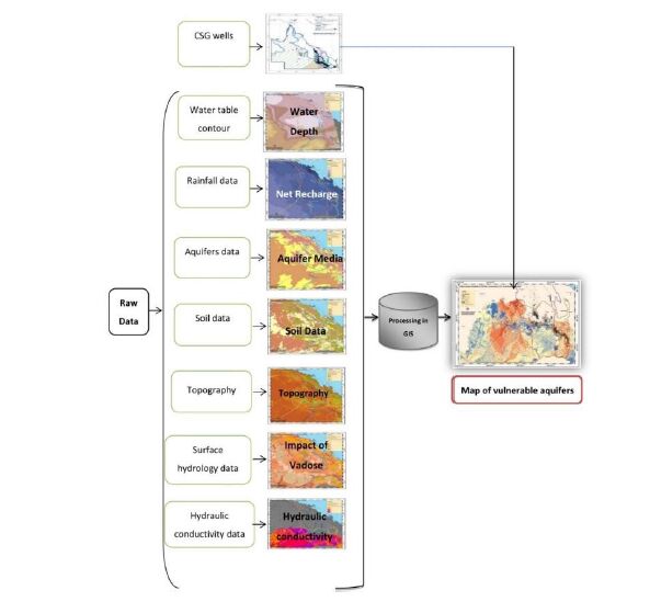 Figure 1. DRASTIC methodology for identifying intrinsic aquifer vulnerability using GIS and indirect estimate of releases using CSG well location.
| Drastic themes | Title | Organisation | Link |
| Aquifer media | Layer name: AHGFWaterTableAquifer, Geospatial Aquifer | Australian Bureau of Meteorology | ftp://ftp.bom.gov.au/anon/home/geofabric |
| Hydraulic conductivity | GeoFabric (V2.0.1) | Australian Bureau of Meteorology | ftp://ftp.bom.gov.au/anon/home/geofabric |
| Impact of Vadose | Layer name: AHGFSurficialHydrogeologicUnit, GeoFabric Surficial/SURFACE GEOLOGY OF AUSTRALIA 2.5MSCALE, 2010 EDITION | Australian Bureau of Meteorology/Geoscience Australia | ftp://ftp.bom.gov.au/anon/home/geofabric https://www.ga.gov.au/products/servlet/controller?event=DEFINE_PRODUCTS |
| Precipitation | Climate, Rain Fall/ National Surface Water | Australian Bureau of Meteorology | http://www.bom.gov.au/jsp/ncc/climate_averages/rainfall/index.jsp |
| Soil media | Digital Soil Atlas | The Commonwealth Scientific and Industrial Research Organisation (CSIRO) | http://www.asris.csiro.au/downloads/Atlas/soilAtlas2M.zip |
| Topography | Digital Elevation Model (DEM) | Geoscience Australia | https://data.qld.gov.au/dataset/digital-elevation-model-3-second-queensland |
| Water table depth | Layer name: AHGFAquiferContour, GeoFabric (V2.0.1 ), | Australian Bureau of Meteorology | ftp://ftp.bom.gov.au/anon/home/geofabric |
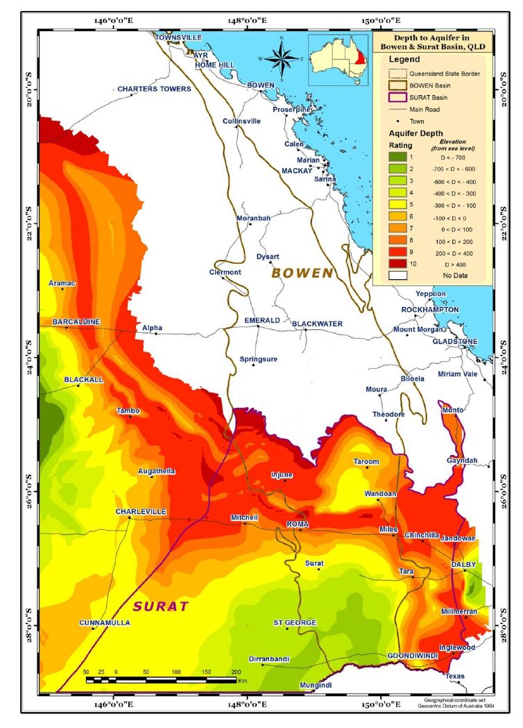
DownLoad: CSVAquifer depth is elevation above sea level (m) obtained from Australian Bureau of Meteorology (BOM). Data for this parameter was not available for the whole region (Figure 2).
The net recharge is the amount of precipitation that migrates into the groundwater. Data on rainfall and evaporation were obtained from BOM and reported as millimetres per year(Figure 3). Net recharge then was calculated as the difference between rainfall and evaporation values [26]. These values were classified into ranges and then assigned ratings from 1 to 10 (Table 3).
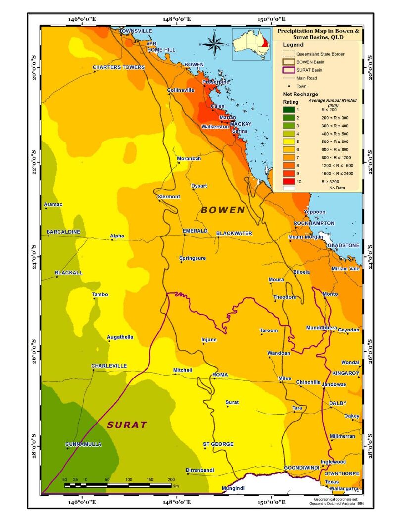 Figure 3. Precipitation climatology for the Bowen and Surat Basins, Queensland—average annual rainfall (mm) [25].
Net recharge value = rainfall−evapotranspiration
The net recharge parameter is then formed from a product of a net recharge rate and a net recharge weight as you can see in drastic index below.
| Feature | Weight | Range | Rating |
| Depth to aquifer (metre) | 5 | D < −700 | 1 |
| −700 < D < −600 | 2 | ||
| −400 < D < −600 | 3 | ||
| −400 < D < −300 | 4 | ||
| −300 < D < −100 | 5 | ||
| −100 < D < 0 | 6 | ||
| 0 < D < 100 | 7 | ||
| 100 < D < 200 | 8 | ||
| 200 < D < 400 | 9 | ||
| D > 400 | 10 | ||
| Net recharge | 4 | R ≤ 200 | 1 |
| 200 < R ≤ 300 | 2 | ||
| 300 < R ≤ 400 | 3 | ||
| 400 < R ≤ 500 | 4 | ||
| 500 < R ≤ 600 | 5 | ||
| 600 < R ≤ 800 | 6 | ||
| 800 < R ≤ 1200 | 7 | ||
| 1200 < R ≤ 1600 | 8 | ||
| 1600 < R ≤ 2400 | 9 | ||
| R ≥ 3200 | 10 | ||
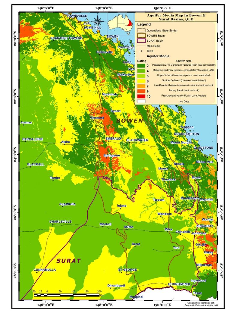
| Aquifer media | 3 | Palaeozoic and Pre-Cambrian Fractured Rock Aquifers (low permeability) | 2 |
| Mesozoic Sediment Aquifer (porous media - consolidated)/Mesozoic (GAB) | 4 | ||
| Upper Tertiary/Quaternary Aquifer (porous media - unconsolidated) | 5 | ||
| Surficial Sediment Aquifer (porous media - unconsolidated) | 6 | ||
| Jurassic (GAB intake beds) (porous media - consolidated) | |||
| Late Permian/Triassic intrusives and volcanics fractured rock aquifers | 7 | ||
| Tertiary Basalt Aquifer (fractured rock) | 9 | ||
| Fractured and Karstic Rocks, Local Aquifers | 10 | ||
| Feature | Weight | Range | Rating |
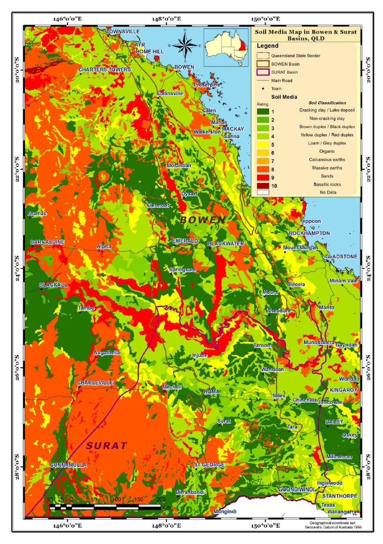
| Soil mediaa | 2 | Cracking clay/Lake deposit | 1 |
| Non-cracking clay | 2 | ||
| Brown duplex/Black duplex | 3 | ||
| Yellow duplex/Red duplex | 4 | ||
| Loam/Gley duplex | 5 | ||
| Organic | 6 | ||
| Calcareous earths | 7 | ||
| Massive earths | 8 | ||
| Sands | 9 | ||
| Basaltic rocks | 10 | ||
| Topography (slope percentage) |
1 | >18 | 1 |
| 12-18 | 3 | ||
| 6-12 | 5 | ||
| 2-6 | 9 | ||
| 0-2 | 10 | ||
| Impact of vadose zone | 5 | Mudstone, siltstone/Claystone/Lacustrine sediment/ | 1 |
| Estuarine sediment/Sinter | 2 | ||
| Mudstone, shale, coal, arenite, argillite, chert | 3 | ||
| Dacite, dolerite, monzogranite/Andesite/Mafic rock/Granite/Teschenite/gabbro gneiss, tuff/Trondhjemite | 4 | ||
| Sandstone/Quartzite, greywacke, amphibolite, chalcedony | 5 | ||
| Limestone/Colluvial sediment/Dolostone | 6 | ||
| Conglomerate, sandstone, Rhyolite/Soil/Alluvial sediment | 7 | ||
| Sand aeolian, beach & coastal sediments | 8 | ||
| Lateritic duricrust, basalt | 9 | ||
| Fractured rock, breccia, volcanic | 10 | ||
| Hydraulic conductivity | 3 | <0.01 | 1 |
| 0.5 | 2 | ||
| 1 | 4 | ||
| 5 | 6 | ||
| 10 | 8 | ||
| 25 >50 |
9 10 |
DownLoad: CSVAquifer media, the rock formation of the aquifer, e.g., sandstone or limestone, is used as a measure of permeability (BOM, Figure 4). Soil media is the upper weathered zone parameter used to indicate the amount of recharge that can infiltrate into the ground. The data for this parameter was obtained from CSIRO (Figure 5). Slope controls the likelihood of water runoff or remaining on the surface. Areas with a low slope allow greater infiltration of recharge, slope percentages for the study area were calculated using the DEM data obtained from Geoscience Australia (Figure 6). The "Impact of vadose zone" is indicated by the lithological units overlying the aquifer and was obtained from BOM (Figure 7). Hydraulic conductivity is the ability of aquifer formation to transmit water. Data for this parameter were obtained from the Australian hydrological geospatial fabric (Geofabric). There were gaps in hydraulic conductivity data for the northern region of the study area (Figure 8).
 Figure 6. Slope—areas with low slope allow greater infiltration of recharge, slope percentages for the study area were calculated using data obtained from Geoscience Australia [28].
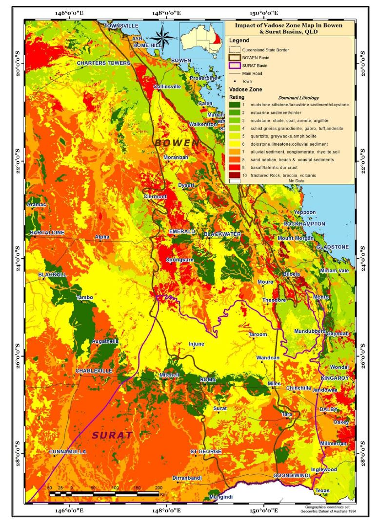 Figure 7. Impact of vadose zone—lithologic units used as a measure of the impact of the vadose zone [24].
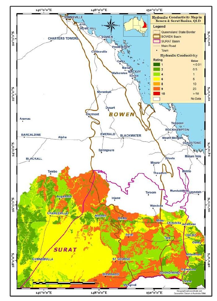 Figure 8. Hydraulic conductivity—the ability of aquifer formation to transmit water (m/day), but not available for northern parts of the basin [24].
Each parameter has a weight that shows its relative importance with respect to the other parameters. Also, each parameter is classified into ranges of values and each range is ranked to indicate the relative importance of that range (Table 3). Ranges and weights were derived based on Aller et al. (1987). A DRASTIC ‘index', which defines the algebra of the method as follows:
Drastic Index =DrDw + RrRw + ArAw + SrSw + TrTw + IrIw + CrCw
where, Dr: rate for Depth to water; Dw: weight for Depth to water;
Rr: rate for net Recharge; Rw: weight for net Recharge;
Ar: rate for Aquifer media; Aw: weight for Aquifer media;
Tr: rate for Topography; Tw: weight for Topography;
Ir: rate for Impact of vadose zone; Iw: weight for Impact of vadose zone;
Cr: rate for hydraulic Conductivity; Cw: weight for hydraulic Conductivity.
The value ranges for some model parameters [23] have been modified to better represent their hydrogeological characteristics in Queensland. For example, depth to water is presented as an estimated depth of drilling to reach the water table [23], but it is reported with respect to sea level in Queensland.
Ranges and their respective rankings for each parameter are displayed along with their weights for DRASTIC parameters (Table 3), the higher the value for the DRASTIC index, the greater the vulnerability of that aquifer location. Maps for seven parameter layers that provided the input to the modelling of vulnerable aquifers were created in GIS (Figures 2-8).
All seven parameter layers were converted into grids for geo-processing, and a groundwater vulnerability map was generated by multiplying each map layer by their corresponding weighting factor.Hydraulic conductivity and depth to aquifer were not available in the northern region of the study area, consequently no vulnerability assessment was possible in these areas (Figure 2 and 8).
ESRI ArcGIS 9.3 software was used to create maps of seven DRASTIC parameters in this assessment. These layers provided the input to the modelling of vulnerable aquifers. A final map of DRASTIC aquifer vulnerability for the study area was developed using the ArcGIS Spatial Analyst tools and processed by raster calculation module. ArcGIS 9.3 software provided an efficient platform for assessing and analysing the vulnerability to groundwater pollution.
Thematic map design strategy was employed in this study, allowing colour ramp tools to classify distinctive data themes. Thematic classification started with standard colour spectrum from green for the lowest rating value, to yellow for medium, red for the highest and white for no data available region. The cartographic documentincludes seven 1:4 million scale hydrogeological parameter maps; a final 1:3.5 million scale map of shallow aquifer vulnerability and an overall map of aquifer vulnerability data layer overlaid with population. In the final map, the change in vulnerability of aquifer is represented by colour and is consistent in each map (red more vulnerable to green less vulnerable). Populations are represented by bar graph symbols on the vulnerability map.
The most vulnerable aquifers are along the east and west margins of the Surat basin (Figure 9), because the hydrological properties are more conducive to the migration of contaminants from surface into groundwater. In the centre of the Surat Basin, groundwater is better protected from contamination by its natural hydrological properties. CSG wells are shown in the map assuming the area where unplanned release of CSG water is more likely to take place (since no data was found about the likelihood of occurrence, volume and location of such unplanned releases). Most CSG wells are found in the eastern and northern areas of the Surat Basin where more vulnerable aquifers can be seen in the east of basin. However, this analysis does not cover the northern end of the basin due to the data gaps in hydraulic conductivity and depth to aquifer.
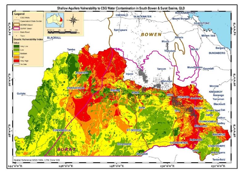 Figure 9. Map of Shallow aquifer vulnerability in the Surat Basin.
Furthermore, it appears that more than 10,000 people live in these areas where the groundwater vulnerability to contamination is high to very high (Figure 10,Table 4). Children and elderly people comprise about one-third of the population. It is assumed that people who are living on top of the aquifers are the potential exposed population, in the event of aquifer contamination.
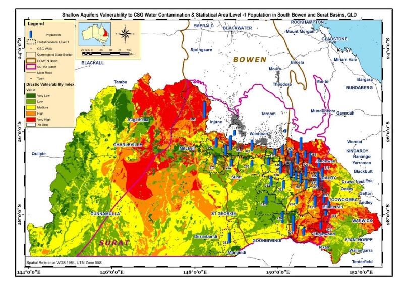 Figure 10. Map of vulnerable shallow aquifers overlaid with potential exposed population—population data obtained from ABS [29].
| Location | Number of people | Number of CSG wells | DRASTIC Vulnerability index |
| Chinchilla | 1529 | 269 | High and very high |
| Goondiwindi | 605 | 2 | |
| Inglewood-Waggamba | 524 | 5 | |
| Miles-Wandoan | 1205 | 989 | |
| Roma Region | 1183 | 1016 | |
| Tara | 1816 | 419 | |
| Millmerran | 1142 | 72 | |
| Wambo | 1347 | 848 | |
| Total | 9351 | 3620 | |
| Balonne | 383 | 1 | Medium |
| Inglewood-Waggamba | 420 | 30 | |
| Miles-Wandoan | 217 | 25 | |
| Roma Region | 1621 | 132 | |
| Tara | 279 | 12 | |
| Total | 2920 | 200 | |
| Miles-Wandoan | 249 | 4 | Low and very low |
| Roma | 376 | 1 | |
| Tara | 986 | 26 | |
| Total | 1611 | 31 | |
| Totals | 13, 882 | 3851 |
DownLoad: CSVThis analysis suggests aquifers with the highest vulnerability are distributed in the east and in the north-west of the Surat basin. However, identification of aquifer vulnerability in the far north and north-east of the basin was not possible due to the absence of data. The geographical distribution of CSG wells shows that there is more CSG activity in the east and north of the basin, while aquifers in the east of the Surat Basin are at higher risk of contamination compared with those in other areas. More than 10,000 people live in the areas with the highest aquifer vulnerability to contamination.
In the event of groundwater aquifer contamination, the environmental health implications will be longer term and more difficult to monitor that would be the case for surface water contamination. To manage this potential problem, more detailed risk assessments should be undertaken. However, except where surface releases of extracted CSG water are explicitly allowed, accidental releases of CSG water are likely to be of greatest concern and control systems failure of pumping, pipelines and/or treatment facilities will need to be evaluated.
The analysis in this study provides a broad scale view of aquifer vulnerability and illustrates the limited data available on the location of releases, their frequency, duration, or chemical concentration in the water. These limit the interpretation of a ‘contamination source map' and the consequent groundwater contamination risk map. However, these research findings might be a useful template for industries and regulators to evaluate the overall potential for groundwater aquifer contamination. Also, considering that the cost of remediating a contaminated aquifer is much higher than maintaining the existing fresh sources, these findings can be used by planners to prioritise monitoring during environmental health risk assessment projects. We suggest that this method should be used prior to approving CSG exploration activities, as a tool for the environmental health risk assessment.
The lack of depth to aquifer and hydraulic conductivity data coverage make it impossible to calculate DRASTIC for the entire Surat and Bowen basins. Information on the volume and location of unplanned releases and geographic distribution of contaminants is limited. Therefore the geographic distribution of CSG wells are overlaid with intrinsic vulnerability maps assuming such incidents are likely to occur near the wells, which may not always be the case. Also, the general lack of an overall consolidated monitoring database inhibits our ability to visualise the geographic distribution of contaminants and combine them with intrinsic vulnerability. While this research cannot estimate risk, it can provide recommendations for future work on generating CSG water sample database and incident inventory for Queensland.
M Navi would like to thank Dr Taulis, QUT, for introducing her to the DRASTIC model.
The authors declare there is no conflict of interest.
| [1] | Nature, 406 (2000), 378-382. |
| [2] | Pharmacy and Therapeutics, 36 (2011), 225-227. |
| [3] | Algorithmica, 40 (2004), 51-62. |
| [4] | Cambridge University Press, Cambridge, 2001. |
| [5] | Proc. Natl. Acad. Sci. USA, 109 (2012), 9209-9212. |
| [6] | Expert Opin. Drug Discov., 8 (2013), 7-20. |
| [7] | Pharmacol. Therapeut., 138 (2013), 333-408. |
| [8] | Symmetry, 2 (2010), 1683-1709, arXiv:1006.3923. |
| [9] | Nat. Rev. Drug Discov., 10 (2011), 563-564. |
| [10] | Nucleic Acid Res., 37 (2009), 1-13. |
| [11] | Nature Protocols, 4 (2009), 44-57, http://david.abcc.ncifcrf.gov/ |
| [12] | John Wiley & Sons, Hoboken, NJ, 2008. |
| [13] | Nucleic Acid Res., 28 (2000), 23-30, http://www.genome.jp/kegg/. |
| [14] | Nucleic Acid Res., 32 (2004), D277-D280. |
| [15] | In A Voronkov, editor, The Alan Turing Centenary, pages 181-195. EasyChair, 2012,http://vlsicad.eecs.umich.edu/BK/SAUCY/. |
| [16] | Computer Science Review, 3 (2009), 199-243. |
| [17] | Landes Bioscience, Austin, TX, 2006. |
| [18] | Springer Verlag, Dordrecht, Heidelberg, New York, London, 2012. |
| [19] | Discr. Appl. Math., 156 (2008), 3525-3531. |
| [20] | http://seer.cancer.gov/. |
| [21] | Theor. Biol. Med. Model., 8 (2011), p21. |
| [22] | Genome Res., 13 (2003), 2498-2504. http://cytoscape.org. |
| [23] | BioSystems, 113 (2013), 149-154. |
| [24] | University of St Andrews, St Andrews, United Kingdom, 2013. http://www.gap-system.org. |
| [25] | BMC Syst. Biol., 7 (2013), p90. |
| [26] | Phys. Rev. E, 78 (2008), 046102, arXiv:0802.4318. |
| [27] | Bioinformatics, 25 (2009), 1470-1471, http://bioconductor.org. |
| 1. | Surina Esterhuyse, Developing a groundwater vulnerability map for unconventional oil and gas extraction: a case study from South Africa, 2017, 76, 1866-6280, 10.1007/s12665-017-6961-6 |

Peter Hinow, Edward A. Rietman, Sara Ibrahim Omar, Jack A. Tuszyński. Algebraic and topological indices of molecular pathway networks in human cancers[J]. Mathematical Biosciences and Engineering, 2015, 12(6): 1289-1302. doi: 10.3934/mbe.2015.12.1289

| Aquifers | Agriculture | Industrial | Urban | S&D | Total |
| Condamine River Alluvium | 41,450 | 550 | 4400 | 8600 | 55,000 |
| Springbok Sandstone | 220 | 351 | 1143 | 1714 | |
| Walloon Coal Measures | 7150 | 594 | 143 | 9040 | 16,927 |
| Hutton & Marburg Sandstones | 8804 | 3698 | 3049 | 12,710 | 28,261 |
| Bungil Formation and Mooga Sandstone | 417 | 1 | 239 | 8418 | 9075 |
| Orallo Formation | 30 | 300 | 330 | ||
| Gubberamunda Sandstone | 2853 | 800 | 1122 | 9047 | 13,822 |
| Rolling Downs Group | 100 | 1050 | 1150 | ||
| Moolayember Formation | 433 | 433 | |||
| Totals | 61,024 | 5643 | 9304 | 50741 | 126,712 |
DownLoad: CSV| Drastic themes | Title | Organisation | Link |
| Aquifer media | Layer name: AHGFWaterTableAquifer, Geospatial Aquifer | Australian Bureau of Meteorology | ftp://ftp.bom.gov.au/anon/home/geofabric |
| Hydraulic conductivity | GeoFabric (V2.0.1) | Australian Bureau of Meteorology | ftp://ftp.bom.gov.au/anon/home/geofabric |
| Impact of Vadose | Layer name: AHGFSurficialHydrogeologicUnit, GeoFabric Surficial/SURFACE GEOLOGY OF AUSTRALIA 2.5MSCALE, 2010 EDITION | Australian Bureau of Meteorology/Geoscience Australia | ftp://ftp.bom.gov.au/anon/home/geofabric https://www.ga.gov.au/products/servlet/controller?event=DEFINE_PRODUCTS |
| Precipitation | Climate, Rain Fall/ National Surface Water | Australian Bureau of Meteorology | http://www.bom.gov.au/jsp/ncc/climate_averages/rainfall/index.jsp |
| Soil media | Digital Soil Atlas | The Commonwealth Scientific and Industrial Research Organisation (CSIRO) | http://www.asris.csiro.au/downloads/Atlas/soilAtlas2M.zip |
| Topography | Digital Elevation Model (DEM) | Geoscience Australia | https://data.qld.gov.au/dataset/digital-elevation-model-3-second-queensland |
| Water table depth | Layer name: AHGFAquiferContour, GeoFabric (V2.0.1 ), | Australian Bureau of Meteorology | ftp://ftp.bom.gov.au/anon/home/geofabric |
DownLoad: CSV| Feature | Weight | Range | Rating |
| Depth to aquifer (metre) | 5 | D < −700 | 1 |
| −700 < D < −600 | 2 | ||
| −400 < D < −600 | 3 | ||
| −400 < D < −300 | 4 | ||
| −300 < D < −100 | 5 | ||
| −100 < D < 0 | 6 | ||
| 0 < D < 100 | 7 | ||
| 100 < D < 200 | 8 | ||
| 200 < D < 400 | 9 | ||
| D > 400 | 10 | ||
| Net recharge | 4 | R ≤ 200 | 1 |
| 200 < R ≤ 300 | 2 | ||
| 300 < R ≤ 400 | 3 | ||
| 400 < R ≤ 500 | 4 | ||
| 500 < R ≤ 600 | 5 | ||
| 600 < R ≤ 800 | 6 | ||
| 800 < R ≤ 1200 | 7 | ||
| 1200 < R ≤ 1600 | 8 | ||
| 1600 < R ≤ 2400 | 9 | ||
| R ≥ 3200 | 10 | ||
| Aquifer media | 3 | Palaeozoic and Pre-Cambrian Fractured Rock Aquifers (low permeability) | 2 |
| Mesozoic Sediment Aquifer (porous media - consolidated)/Mesozoic (GAB) | 4 | ||
| Upper Tertiary/Quaternary Aquifer (porous media - unconsolidated) | 5 | ||
| Surficial Sediment Aquifer (porous media - unconsolidated) | 6 | ||
| Jurassic (GAB intake beds) (porous media - consolidated) | |||
| Late Permian/Triassic intrusives and volcanics fractured rock aquifers | 7 | ||
| Tertiary Basalt Aquifer (fractured rock) | 9 | ||
| Fractured and Karstic Rocks, Local Aquifers | 10 | ||
| Feature | Weight | Range | Rating |
| Soil mediaa | 2 | Cracking clay/Lake deposit | 1 |
| Non-cracking clay | 2 | ||
| Brown duplex/Black duplex | 3 | ||
| Yellow duplex/Red duplex | 4 | ||
| Loam/Gley duplex | 5 | ||
| Organic | 6 | ||
| Calcareous earths | 7 | ||
| Massive earths | 8 | ||
| Sands | 9 | ||
| Basaltic rocks | 10 | ||
| Topography (slope percentage) |
1 | >18 | 1 |
| 12-18 | 3 | ||
| 6-12 | 5 | ||
| 2-6 | 9 | ||
| 0-2 | 10 | ||
| Impact of vadose zone | 5 | Mudstone, siltstone/Claystone/Lacustrine sediment/ | 1 |
| Estuarine sediment/Sinter | 2 | ||
| Mudstone, shale, coal, arenite, argillite, chert | 3 | ||
| Dacite, dolerite, monzogranite/Andesite/Mafic rock/Granite/Teschenite/gabbro gneiss, tuff/Trondhjemite | 4 | ||
| Sandstone/Quartzite, greywacke, amphibolite, chalcedony | 5 | ||
| Limestone/Colluvial sediment/Dolostone | 6 | ||
| Conglomerate, sandstone, Rhyolite/Soil/Alluvial sediment | 7 | ||
| Sand aeolian, beach & coastal sediments | 8 | ||
| Lateritic duricrust, basalt | 9 | ||
| Fractured rock, breccia, volcanic | 10 | ||
| Hydraulic conductivity | 3 | <0.01 | 1 |
| 0.5 | 2 | ||
| 1 | 4 | ||
| 5 | 6 | ||
| 10 | 8 | ||
| 25 >50 |
9 10 |
DownLoad: CSV| Location | Number of people | Number of CSG wells | DRASTIC Vulnerability index |
| Chinchilla | 1529 | 269 | High and very high |
| Goondiwindi | 605 | 2 | |
| Inglewood-Waggamba | 524 | 5 | |
| Miles-Wandoan | 1205 | 989 | |
| Roma Region | 1183 | 1016 | |
| Tara | 1816 | 419 | |
| Millmerran | 1142 | 72 | |
| Wambo | 1347 | 848 | |
| Total | 9351 | 3620 | |
| Balonne | 383 | 1 | Medium |
| Inglewood-Waggamba | 420 | 30 | |
| Miles-Wandoan | 217 | 25 | |
| Roma Region | 1621 | 132 | |
| Tara | 279 | 12 | |
| Total | 2920 | 200 | |
| Miles-Wandoan | 249 | 4 | Low and very low |
| Roma | 376 | 1 | |
| Tara | 986 | 26 | |
| Total | 1611 | 31 | |
| Totals | 13, 882 | 3851 |
DownLoad: CSV| Aquifers | Agriculture | Industrial | Urban | S&D | Total |
| Condamine River Alluvium | 41,450 | 550 | 4400 | 8600 | 55,000 |
| Springbok Sandstone | 220 | 351 | 1143 | 1714 | |
| Walloon Coal Measures | 7150 | 594 | 143 | 9040 | 16,927 |
| Hutton & Marburg Sandstones | 8804 | 3698 | 3049 | 12,710 | 28,261 |
| Bungil Formation and Mooga Sandstone | 417 | 1 | 239 | 8418 | 9075 |
| Orallo Formation | 30 | 300 | 330 | ||
| Gubberamunda Sandstone | 2853 | 800 | 1122 | 9047 | 13,822 |
| Rolling Downs Group | 100 | 1050 | 1150 | ||
| Moolayember Formation | 433 | 433 | |||
| Totals | 61,024 | 5643 | 9304 | 50741 | 126,712 |
| Drastic themes | Title | Organisation | Link |
| Aquifer media | Layer name: AHGFWaterTableAquifer, Geospatial Aquifer | Australian Bureau of Meteorology | ftp://ftp.bom.gov.au/anon/home/geofabric |
| Hydraulic conductivity | GeoFabric (V2.0.1) | Australian Bureau of Meteorology | ftp://ftp.bom.gov.au/anon/home/geofabric |
| Impact of Vadose | Layer name: AHGFSurficialHydrogeologicUnit, GeoFabric Surficial/SURFACE GEOLOGY OF AUSTRALIA 2.5MSCALE, 2010 EDITION | Australian Bureau of Meteorology/Geoscience Australia | ftp://ftp.bom.gov.au/anon/home/geofabric https://www.ga.gov.au/products/servlet/controller?event=DEFINE_PRODUCTS |
| Precipitation | Climate, Rain Fall/ National Surface Water | Australian Bureau of Meteorology | http://www.bom.gov.au/jsp/ncc/climate_averages/rainfall/index.jsp |
| Soil media | Digital Soil Atlas | The Commonwealth Scientific and Industrial Research Organisation (CSIRO) | http://www.asris.csiro.au/downloads/Atlas/soilAtlas2M.zip |
| Topography | Digital Elevation Model (DEM) | Geoscience Australia | https://data.qld.gov.au/dataset/digital-elevation-model-3-second-queensland |
| Water table depth | Layer name: AHGFAquiferContour, GeoFabric (V2.0.1 ), | Australian Bureau of Meteorology | ftp://ftp.bom.gov.au/anon/home/geofabric |
| Feature | Weight | Range | Rating |
| Depth to aquifer (metre) | 5 | D < −700 | 1 |
| −700 < D < −600 | 2 | ||
| −400 < D < −600 | 3 | ||
| −400 < D < −300 | 4 | ||
| −300 < D < −100 | 5 | ||
| −100 < D < 0 | 6 | ||
| 0 < D < 100 | 7 | ||
| 100 < D < 200 | 8 | ||
| 200 < D < 400 | 9 | ||
| D > 400 | 10 | ||
| Net recharge | 4 | R ≤ 200 | 1 |
| 200 < R ≤ 300 | 2 | ||
| 300 < R ≤ 400 | 3 | ||
| 400 < R ≤ 500 | 4 | ||
| 500 < R ≤ 600 | 5 | ||
| 600 < R ≤ 800 | 6 | ||
| 800 < R ≤ 1200 | 7 | ||
| 1200 < R ≤ 1600 | 8 | ||
| 1600 < R ≤ 2400 | 9 | ||
| R ≥ 3200 | 10 | ||
| Aquifer media | 3 | Palaeozoic and Pre-Cambrian Fractured Rock Aquifers (low permeability) | 2 |
| Mesozoic Sediment Aquifer (porous media - consolidated)/Mesozoic (GAB) | 4 | ||
| Upper Tertiary/Quaternary Aquifer (porous media - unconsolidated) | 5 | ||
| Surficial Sediment Aquifer (porous media - unconsolidated) | 6 | ||
| Jurassic (GAB intake beds) (porous media - consolidated) | |||
| Late Permian/Triassic intrusives and volcanics fractured rock aquifers | 7 | ||
| Tertiary Basalt Aquifer (fractured rock) | 9 | ||
| Fractured and Karstic Rocks, Local Aquifers | 10 | ||
| Feature | Weight | Range | Rating |
| Soil mediaa | 2 | Cracking clay/Lake deposit | 1 |
| Non-cracking clay | 2 | ||
| Brown duplex/Black duplex | 3 | ||
| Yellow duplex/Red duplex | 4 | ||
| Loam/Gley duplex | 5 | ||
| Organic | 6 | ||
| Calcareous earths | 7 | ||
| Massive earths | 8 | ||
| Sands | 9 | ||
| Basaltic rocks | 10 | ||
| Topography (slope percentage) |
1 | >18 | 1 |
| 12-18 | 3 | ||
| 6-12 | 5 | ||
| 2-6 | 9 | ||
| 0-2 | 10 | ||
| Impact of vadose zone | 5 | Mudstone, siltstone/Claystone/Lacustrine sediment/ | 1 |
| Estuarine sediment/Sinter | 2 | ||
| Mudstone, shale, coal, arenite, argillite, chert | 3 | ||
| Dacite, dolerite, monzogranite/Andesite/Mafic rock/Granite/Teschenite/gabbro gneiss, tuff/Trondhjemite | 4 | ||
| Sandstone/Quartzite, greywacke, amphibolite, chalcedony | 5 | ||
| Limestone/Colluvial sediment/Dolostone | 6 | ||
| Conglomerate, sandstone, Rhyolite/Soil/Alluvial sediment | 7 | ||
| Sand aeolian, beach & coastal sediments | 8 | ||
| Lateritic duricrust, basalt | 9 | ||
| Fractured rock, breccia, volcanic | 10 | ||
| Hydraulic conductivity | 3 | <0.01 | 1 |
| 0.5 | 2 | ||
| 1 | 4 | ||
| 5 | 6 | ||
| 10 | 8 | ||
| 25 >50 |
9 10 |
| Location | Number of people | Number of CSG wells | DRASTIC Vulnerability index |
| Chinchilla | 1529 | 269 | High and very high |
| Goondiwindi | 605 | 2 | |
| Inglewood-Waggamba | 524 | 5 | |
| Miles-Wandoan | 1205 | 989 | |
| Roma Region | 1183 | 1016 | |
| Tara | 1816 | 419 | |
| Millmerran | 1142 | 72 | |
| Wambo | 1347 | 848 | |
| Total | 9351 | 3620 | |
| Balonne | 383 | 1 | Medium |
| Inglewood-Waggamba | 420 | 30 | |
| Miles-Wandoan | 217 | 25 | |
| Roma Region | 1621 | 132 | |
| Tara | 279 | 12 | |
| Total | 2920 | 200 | |
| Miles-Wandoan | 249 | 4 | Low and very low |
| Roma | 376 | 1 | |
| Tara | 986 | 26 | |
| Total | 1611 | 31 | |
| Totals | 13, 882 | 3851 |