Contribution of morphological study to the understanding of watersheds in arid environment: A case study (Morocco)

Mounir OUABA; Mohamed Elmehdi SAIDI; Mounir OUABA; Mohamed Elmehdi SAIDI

doi:10.3934/environsci.2023002

AIMS Environmental Science

2023, Volume 10, Issue 1: 16-32. doi: 10.3934/environsci.2023002

Previous Article Next Article

Research article

Contribution of morphological study to the understanding of watersheds in arid environment: A case study (Morocco)

Mounir OUABA ^,,
Mohamed Elmehdi SAIDI

Georesources, Geoenvironment and Civil Engineering Laboratory, Cadi Ayyad University, Marrakech 40000, Morocco

Received: 19 July 2022 Revised: 13 September 2022 Accepted: 20 September 2022 Published: 08 November 2022

Watershed planning is often based on the analysis of morphometric parameters, especially in poorly gauged or ungauged basins. These physiographic parameters have, in fact, a main role in water runoff. In many arid countries such as Morocco, there is a significant need for morphometric studies of watersheds to initiate integrated water resources management. For this purpose, we have carried out the watersheds delineation and morphometric analyses, using the Digital Terrain Model (DTM) and the Geographic Information System (GIS). We have applied this approach based on remote sensing and GIS in four sub-basins of the right bank of the Tensift watershed (Bourrous, Al Wiza, El Hallouf and Jamala). The shape indexes of Gravelius and Horton reveal elongated shapes of the four watersheds. In addition, the maximum slope and the drainage density do not exceed 27.15° and 1 Km/Km² respectively. The sub-basins do not have a very dense hydrographic network and the Strahler's drainage order is not very high (up to 5). The relief is not very high and do not reach 1000 m. These physiographic conditions do not allow a rapid runoff. The concentration times are precisely quite high (7 to 12 hours for watersheds of 161 to 401 km²). The use of a sufficiently fine DTM resolution and an appropriate GIS software would allow this kind of study to be very useful for effective watershed management.
- watershed morphometry,
- Digital Terrain Model,
- GIS,
- arid environment,
- Morocco
Citation: Mounir OUABA, Mohamed Elmehdi SAIDI. Contribution of morphological study to the understanding of watersheds in arid environment: A case study (Morocco)[J]. AIMS Environmental Science, 2023, 10(1): 16-32. doi: 10.3934/environsci.2023002

Related Papers:

Abstract

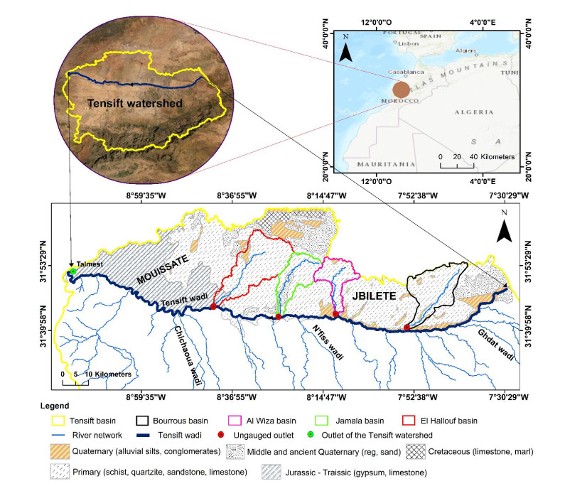
Watershed planning is often based on the analysis of morphometric parameters, especially in poorly gauged or ungauged basins. These physiographic parameters have, in fact, a main role in water runoff. In many arid countries such as Morocco, there is a significant need for morphometric studies of watersheds to initiate integrated water resources management. For this purpose, we have carried out the watersheds delineation and morphometric analyses, using the Digital Terrain Model (DTM) and the Geographic Information System (GIS). We have applied this approach based on remote sensing and GIS in four sub-basins of the right bank of the Tensift watershed (Bourrous, Al Wiza, El Hallouf and Jamala). The shape indexes of Gravelius and Horton reveal elongated shapes of the four watersheds. In addition, the maximum slope and the drainage density do not exceed 27.15° and 1 Km/Km² respectively. The sub-basins do not have a very dense hydrographic network and the Strahler's drainage order is not very high (up to 5). The relief is not very high and do not reach 1000 m. These physiographic conditions do not allow a rapid runoff. The concentration times are precisely quite high (7 to 12 hours for watersheds of 161 to 401 km²). The use of a sufficiently fine DTM resolution and an appropriate GIS software would allow this kind of study to be very useful for effective watershed management.

References

[1]	Li K, Huang G, Wang S (2019) Market-based stochastic optimization of water resources systems for improving drought resilience and economic efficiency in arid regions. J Clean Prod 233: 522–537. https://doi.org/10.1016/j.jclepro.2019.05.379. doi: 10.1016/j.jclepro.2019.05.379
[2]	Pachauri RK, Meyer LA (2014) Climate Change 2014: Synthesis Report. Contribution of Working Groups I, II and III to the Fifth Assessment Report of the Intergovernmental Panel on Climate Change / R. Pachauri and L. Meyer (editors), Geneva, Switzerland, IPCC, 151.
[3]	Zhang X, Xu D, Wang Z (2021) Optimizing spatial layout of afforestation to realize the maximum benefit of water resources in arid regions: A case study of Alxa, China. Journal of Cleaner Production 320: 128827. https://doi.org/10.1016/j.jclepro.2021.128827.30 doi: 10.1016/j.jclepro.2021.128827.30
[4]	Abd-Elaty I, Kuriqi A, Shahawy AE (2022) Environmental rethinking of wastewater drains to manage environmental pollution and alleviate water scarcity. Nat Hazards 110: 2353–2380. https://doi.org/10.1007/s11069-021-05040-w doi: 10.1007/s11069-021-05040-w
[5]	Aly MM, Sakr SA, Zayed MSM (2022) Selection of the optimum locations for rainwater harvesting in arid regions using WMS and remote sensing. Case Study: Wadi Hodein Basin, Red Sea, Egypt. Alexandria Engineering Journal 61: 9795–9810. https://doi.org/10.1016/j.aej.2022.02.046 doi: 10.1016/j.aej.2022.02.046
[6]	Niyazi BA, Masoud MH, Ahmed M, et al. (2020) Runoff Assessment and Modeling in Arid Regions by Integration ofWatershed and Hydrologic Models with GIS Techniques. Journal of African Earth Sciences 172: 103966. https://doi.org/10.1016/j.jafrearsci.2020.103966 doi: 10.1016/j.jafrearsci.2020.103966
[7]	Saha S, Das J, Mandal T (2022) Investigation of the watershed hydro-morphologic characteristics through the morphometric analysis: A study on Rayeng basin in Darjeeling Himalaya. Environmental Challenges 7: 100463. https://doi.org/10.1016/j.envc.2022.100463 doi: 10.1016/j.envc.2022.100463
[8]	Resmi MR, Babeesh C, Achyuthan H (2019) Quantitative analysis of the drainage and morphometric characteristics of the Palar River basin, Southern Peninsular India; using bAd calculator (bearing azimuth and drainage) and GIS. Geology, Ecology, and Landscapes 3: 295–307. https://doi.org/10.1080/24749508.2018.1563750 doi: 10.1080/24749508.2018.1563750
[9]	Mahala A (2020) The significance of morphometric analysis to understand the hydrological and morphological characteristics in two different morpho-climatic settings. Appl Water Sci 10: 33. https://doi.org/10.1007/s13201-019-1118-2 doi: 10.1007/s13201-019-1118-2
[10]	Saidi ME, Daoudi L, Aresmouk MEH, et al. (2010) The Ourika floods (High Atlas, Morocco), extreme events in semi-arid mountain context. Comunicacoes Geologicas 97: 113–128.
[11]	Mazenc, B, Sanchez, M, Thiery, D (1984) Analysis of the influence of the geomorphological characteristics of a river basin on the parameters of a global hydrological model and on the discharge at the outlet. Journal of Hydrology 69: 97–118. https://doi.org/10.1016/0022-1694(84)90158-6 doi: 10.1016/0022-1694(84)90158-6
[12]	Brouziyne Y, Belaqziz S, Benaabidate L, et al. (2022) Modeling long term response of environmental flow attributes to future climate change in a North African watershed (Bouregreg watershed, Morocco). Ecohydrology & Hydrobiology 22: 155–167. https://doi.org/10.1016/j.ecohyd.2021.08.005 doi: 10.1016/j.ecohyd.2021.08.005
[13]	Ahattab J, Serhir N, Lakhal EK (2015) Towards elaboration of a Decision Support System for selection of methods to evaluate flood peaks in Morocco: Readaptation of classic methods to recent hydrological data. La Houille Blanche 101: 63–70. https://doi.org/10.1051/lhb/2015008 doi: 10.1051/lhb/2015008
[14]	Saidi ME, Agoussine M, Daoudi L (2006) Impact of morphology and exposure on the surface water resources in the High Atlas mountains (Morocco): example of the Ourika and Marghene watersheds. Bulletin de l'Institut Scientifique, Rabat, section Sciences de la Terre 28: 41–49.
[15]	Sarkar P, Kumar P, Vishwakarma D, et al. (2022) Watershed prioritization using morphometric analysis by MCDM approaches. Ecological Informatics 70: 101763. https://doi.org/10.1016/j.ecoinf.2022.101763 doi: 10.1016/j.ecoinf.2022.101763
[16]	Doyle FJ (1978) Digital terrain models: an overview. Photogrammetric Engineering and Remote Sensing 44: 1481–1485.
[17]	Guiamel IA, Lee HS (2020) Watershed modelling of the Mindanao River Basin in the Philippines using the SWAT for water resource management. Civil Engineering Journal 6: 626–648. https://doi.org/10.28991/cej-2020-03091496 doi: 10.28991/cej-2020-03091496
[18]	US Geological Survey (1987) Digital elevation models. US Geological Survey Data User's Guide 5: 38.
[19]	Tesema TA (2021) Impact of identical digital elevation model resolution and sources on morphometric parameters of Tena watershed, Ethiopia. Heliyon 7: e08345. https://doi.org/10.1016/j.heliyon.2021.e08345 doi: 10.1016/j.heliyon.2021.e08345
[20]	Chou TY, Lin WT, Lin CY, et al. (2004) Application of the PROMETHEE technique to determine depression outlet location and flow direction in DEM. Journal of Hydrology 287: 49–61. https://doi.org/10.1016/j.jhydrol.2003.09.026 doi: 10.1016/j.jhydrol.2003.09.026
[21]	Farr TG, Kobrick M (2000) Shuttle Radar Topography Mission produces a wealth of data. Eos Trans 81:583–583.
[22]	Farr TG, Rosen, PA, Caro E, et al. (2007) The shuttle radar topography mission. Reviews of geophysics 45. https://doi.org/10.1029/2005RG000183
[23]	Wei C, Dong X, Yu D, et al. (2022) An alternative to the Grain for Green Program for soil and water conservation in the upper Huaihe River basin, China. Journal of Hydrology: Regional Studies 43: 101180. https://doi.org/10.1016/j.ejrh.2022.101180 doi: 10.1016/j.ejrh.2022.101180
[24]	Li S, Sun D, Goldberg M, et al. (2022) A downscaling model for derivation of 3-D flood products from VIIRS imagery and SRTM/DEM. ISPRS Journal of Photogrammetry and Remote Sensing 192: 279–298. https://doi.org/10.1016/j.isprsjprs.2022.08.025 doi: 10.1016/j.isprsjprs.2022.08.025
[25]	Environmental Systems Research Institute (ESRI) Arc Hydro Geoprocessing Tools [Rapport]: Tutorial. - New York: ESRI, 2011.
[26]	Veen CV (2008) ESRI Founder Jack Dangermond Predicts the Future of GIS. Government Technology in California.
[27]	Ouaba M, El Khalki EM, Saidi MEM, et al. (2022) Estimation of flood discharge in ungauged basin using GPM-IMERG satellite-based precipitation dataset in Moroccan arid zone. Earth Systems and Environment 2022: 1–16. https://doi.org/10.1007/s41748-022-00296-z doi: 10.1007/s41748-022-00296-z
[28]	Noudja T, Wonkam C, Kalédjé PSK, et al. (2022) Updating morphometric features and their accuracy: a case study of the Sanaga watershed in Cameroon. Arab J Geosci 15: 274. https://doi.org/10.1007/s12517-022-09506-4 doi: 10.1007/s12517-022-09506-4
[29]	Arabameri A, Tiefenbacher JP, Blaschke T, et al. (2020) Morphometric Analysis for Soil Erosion Susceptibility Mapping Using Novel GIS-Based Ensemble Model. Remote Sensing 12: 874. https://doi.org/10.3390/rs12050874 doi: 10.3390/rs12050874
[30]	Cochet A (1975) Water resources of Morocco (Ressources en eau du Maroc). Tome 2. The Atlantic plain and basin. Edition of the geological service of Morocco 1975: 393–397.
[31]	NASA Shuttle Radar Topography Mission (SRTM) (2013) Shuttle Radar Topography Mission (SRTM) Global. Distributed by OpenTopography. https://doi.org/10.5069/G9445JDF.Accessed: 2022-07-13
[32]	Gravelius H (1914) The basic principles of the entire science of weights and measures (Grundrifi der gesamten Gewcisserkunde). Band I: Flufikunde (Compendium of Hydrology, Vol. I. Rivers, in German). Goschen, Berlin.
[33]	Horton R (1945) Erosional Development of Streams and Their Drainage Basins; Hydrophysical Approach to Quantitative Morphology. Geological Society of America Bulletin 56: 275–370. http://dx.doi.org/10.1130/0016-7606(1945)56[275:EDOSAT]2.0.CO;2 doi: 10.1130/0016-7606(1945)56[275:EDOSAT]2.0.CO;2
[34]	Roche M (1963) Hydrologie de surface. ORSTOM, Gauthier-Villars, Paris.
[35]	Horton RE (1932) Drainage-basin characteristics. Transactions, American Geophysical Union 13: 350. https://doi.org/10.1029/tr013i001p00350 doi: 10.1029/tr013i001p00350
[36]	Strahler A (1964) Quantitative Geomorphology of Drainage Basins and Channel Networks. In: Chow, V., Ed., Handbook of Applied Hydrology, McGraw Hill, New York, 439–476.
[37]	Ouarda TB, Gingras H, Bobée B, et al. (2001) Synthèse des méthodes simples de régionalisation.
[38]	Ahattab J (2016) Readaptation of flood estimation methods to recent extreme hydrological data of the Tensift and Essaouira watersheds (Réadaptation des méthodes d'estimation de crues aux données hydrologiques extrêmes récentes des bassins versants de Tensift et Essaouira). PhD Thesis, University of Cadi Ayyad, Marrakech, Morocco.

Reader Comments

Your name:*

Email:*
© 2023 the Author(s), licensee AIMS Press. This is an open access article distributed under the terms of the Creative Commons Attribution License (http://creativecommons.org/licenses/by/4.0)