Decision models enhancing environmental flow sustainability: A strategic approach to water resource management

Seiran Haghgoo; Jamil Amanollahi; Barzan Bahrami Kamangar; Shahryar Sorooshian; Seiran Haghgoo; Jamil Amanollahi; Barzan Bahrami Kamangar; Shahryar Sorooshian

doi:10.3934/environsci.2024045

AIMS Environmental Science

2024, Volume 11, Issue 6: 900-917. doi: 10.3934/environsci.2024045

Previous Article Next Article

Research article Special Issues

Decision models enhancing environmental flow sustainability: A strategic approach to water resource management

1.
Department of Environmental Sciences, Faculty of Natural Resources, University of Kurdistan, Iran
2.
Department of Fisheries, Faculty of Natural Resources, University of Kurdistan, Iran
3.
Department of Business Administration, University of Gothenburg, Sweden

Received: 27 May 2024 Revised: 26 July 2024 Accepted: 10 October 2024 Published: 16 October 2024

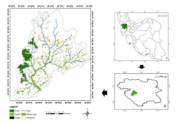
Proper water resource management is essential for maintaining a sustainable supply chain and meeting water demand. The urgent need to preserve river ecosystems by sustaining environmental flow (EF) in the realm of environmental management has been highlighted by the drastic changes to river ecosystems and upstream flow dynamics brought about by careless river exploitation in the last few decades. To optimize EF in river basin management, we present an integrated modeling approach. We focused on the Pir Khezran River basin. Our objective was to estimate EF and generalize the findings to adjacent rivers using modeling techniques, thus providing valuable insights for environmental management applications. The assessment and optimization of EF under uncertain conditions was achieved by combining physical habitat simulation (PHABSIM) modeling with advanced techniques like Adaptive Neuro-Fuzzy Inference Systems (ANFIS) and Multilayer Perceptron (MLP) neural networks. This integrated modeling approach contributes to sustainable solutions for river basin management and environmental conservation by effectively optimizing EF, as demonstrated by the results. This research, therefore, makes valuable contributions to environmental management in various areas such as ecological preservation, modeling and optimizing environmental systems, and policy considerations.

Keywords:

Citation: Seiran Haghgoo, Jamil Amanollahi, Barzan Bahrami Kamangar, Shahryar Sorooshian. Decision models enhancing environmental flow sustainability: A strategic approach to water resource management[J]. AIMS Environmental Science, 2024, 11(6): 900-917. doi: 10.3934/environsci.2024045

Related Papers:

[1]	Zhichao Jiang, Xiaohua Bi, Tongqian Zhang, B.G. Sampath Aruna Pradeep . Global Hopf bifurcation of a delayed phytoplankton-zooplankton system considering toxin producing effect and delay dependent coefficient. Mathematical Biosciences and Engineering, 2019, 16(5): 3807-3829. doi: 10.3934/mbe.2019188
[2]	Ruiqing Shi, Jianing Ren, Cuihong Wang . Stability analysis and Hopf bifurcation of a fractional order mathematical model with time delay for nutrient-phytoplankton-zooplankton. Mathematical Biosciences and Engineering, 2020, 17(4): 3836-3868. doi: 10.3934/mbe.2020214
[3]	Juan Li, Yongzhong Song, Hui Wan, Huaiping Zhu . Dynamical analysis of a toxin-producing phytoplankton-zooplankton model with refuge. Mathematical Biosciences and Engineering, 2017, 14(2): 529-557. doi: 10.3934/mbe.2017032
[4]	Fang Liu, Yanfei Du . Spatiotemporal dynamics of a diffusive predator-prey model with delay and Allee effect in predator. Mathematical Biosciences and Engineering, 2023, 20(11): 19372-19400. doi: 10.3934/mbe.2023857
[5]	Elvira Barbera, Giancarlo Consolo, Giovanna Valenti . A two or three compartments hyperbolic reaction-diffusion model for the aquatic food chain. Mathematical Biosciences and Engineering, 2015, 12(3): 451-472. doi: 10.3934/mbe.2015.12.451
[6]	Zhenyao Sun, Da Song, Meng Fan . Dynamics of a stoichiometric phytoplankton-zooplankton model with season-driven light intensity. Mathematical Biosciences and Engineering, 2024, 21(8): 6870-6897. doi: 10.3934/mbe.2024301
[7]	Kawkab Al Amri, Qamar J. A Khan, David Greenhalgh . Combined impact of fear and Allee effect in predator-prey interaction models on their growth. Mathematical Biosciences and Engineering, 2024, 21(10): 7211-7252. doi: 10.3934/mbe.2024319
[8]	Yuanpei Xia, Weisong Zhou, Zhichun Yang . Global analysis and optimal harvesting for a hybrid stochastic phytoplankton-zooplankton-fish model with distributed delays. Mathematical Biosciences and Engineering, 2020, 17(5): 6149-6180. doi: 10.3934/mbe.2020326
[9]	Kalyan Manna, Malay Banerjee . Stability of Hopf-bifurcating limit cycles in a diffusion-driven prey-predator system with Allee effect and time delay. Mathematical Biosciences and Engineering, 2019, 16(4): 2411-2446. doi: 10.3934/mbe.2019121
[10]	Yuhong Huo, Gourav Mandal, Lakshmi Narayan Guin, Santabrata Chakravarty, Renji Han . Allee effect-driven complexity in a spatiotemporal predator-prey system with fear factor. Mathematical Biosciences and Engineering, 2023, 20(10): 18820-18860. doi: 10.3934/mbe.2023834

Abstract

1. Introduction

Blooms are considered to be a rapid and significant increase in marine phytoplankton populations. It is generally believed that zooplankton is the primary predator of blooms. The zooplankton dissolves phytoplankton blooms in the bud by feeding a large amount of phytoplankton, thereby achieving the purpose of preventing and controlling algal blooms. It is clearly stated in an international research plan that the dynamic changes of zooplankton in marine ecosystems control the change in the total amount of primary productivity. This indicates that zooplankton plays a very important role in the production of phytoplankton and the control of existing quantities. In addition, this is also one of the significant reasons that the interaction between phytoplankton and zooplankton has been widely concerned by many scholars ^{[1,2,3,4,5,6]} in recent years.

Due to the importance of the interaction between phytoplankton and zooplankton in marine biological systems, many scholars have proposed a large number of models to describe this interaction. Moreover, they have continued to study this topic for the past few decades and have achieved very significant results ^{[7,8,9,10,11,12,13]}. Chakraborty et al. ^[7] proposed a mathematical model incorporating nutrient concentration, toxin producing phytoplankton (TPP), non-toxic phytoplankton (NTP), and toxin concentration and explained that TPP species controls the outbreaks of other NTP species when nutrient-deficient conditions are beneficial for the TPP species to release toxin. Saha and Bandyopadhyay ^[8] analyzed a toxin producing phytoplankton-zooplankton model in which the release of toxins from phytoplankton species follows a discrete time variation and discussed the basic dynamics of the system. Banerjee and Venturino ^[9] proposed a phytoplankton-toxic phytoplankton-zooplankton model and found that toxic phytoplankton population does not cause zooplankton population to become extinct. Javidi and Ahmad ^[10] investigated the dynamics of a time fractional order toxic-phytoplankton-phytoplankton-zooplankton system(TPPZS) and did some numerical simulations to validate the theoretical results. Han and Dai ^[11] studied the spatiotemporal pattern caused by cross-diffusion of a toxic-phytoplankton-zooplankton model with nonmonotonic functional response and discussed the effect of toxin-producing rate of toxic-phytoplankton (TPP) species and natural mortality rate of zooplankton species on pattern selection. In addition, Han and Dai proposed a spatiotemporal pattern formation and selection driven by nonlinear cross-diffusion of a toxic-phytoplankton-zooplankton model with Allee effect in ^[12]. Zheng and Sugie ^[13] studied a three-dimensional system including phytoplankton, zooplankton and fish and gave a sufficient condition to ensure that the equilibrium of this three-dimensional system is globally asymptotically stable. Furthermore, they also proved that the equilibrium is asymptotically stable under relatively weak conditions.

Because the seabed has a variety of sediments that can be used as a refuge for the prey, some phytoplankton populations reduce the risk of being caught by zooplankton through refuge. Therefore, some scholars ^{[14,15,16,17,18]} have considered the prey refuge in the predator-prey model in recent years. Kar ^[14] proposed a prey-predator model incorporating a prey refuge and studied the influence of prey refuge on the prey-predator model. Chen and Chen ^[15] investigated a predator-prey model with Holling type Ⅱ functional response incorporating a constant prey refuge and gave the basic dynamical behaviors of the model. Tripathi et al. ^[16] studied a prey-predator model with reserved area and found that the predator species would exist if the value of prey reserve does not exceed a threshold value, beyond which the predator species would become extinct. Ghosh et al. ^[17] analyzed the effect of additional food for predator on the dynamical behaviors of a prey-predator model with prey refuge, they suggested that the possibility of extinction of predator species in high prey refuge ecosystems can be eliminated by providing additional food to predator species. Samanta et al. ^[18] proposed a fractional-order prey-predator model with prey refuge and derived some sufficient conditions to guarantee the global asymptotic stability of predator-extinction equilibrium and co-existing equilibrium.

Li et al. ^[19] considered the factors that phytoplankton protects themselves from being eaten by zooplankton by releasing toxin and taking refuge, and proposed a toxic phytoplankton-zooplankton model with refuge

$\begin{equation} \left\{ \begin{aligned} \overset{.}P(t) & = rP(1-\frac{P}{K})-\frac{\beta_{1}(P-m)}{a_{1}+(P-m)}Z , \\ \overset{.}Z(t) & = \frac{\beta_{2}(P-m)}{a_{1}+(P-m)}Z-dZ-\frac{\theta P}{a_{2}+P}Z , \end{aligned} \right. \end{equation}$

(1.1)

where $P(t)\; \text{and}\; Z(t)$ denote population size of phytoplankton and zooplankton at time $t$ , respectively; $r$ is the intrinsic growth rate; $K$ is the environmental carrying capacity in the absence of zooplankton; $\beta_{1}$ , $\beta_{2}$ $(0 < \beta_{2} < \beta_{1})$ and $d$ describe the predation rate, the ratio of biomass conservation and the natural death rate of zooplankton species, respectively; $a_{1}$ and $a_{2}$ are the half saturation constants; $\theta$ represents the rates of toxin production per phytoplankton species; $m$ is the constant refuge capacity of phytoplankton population, then $P-m$ denotes the number of unprotected phytoplankton is captured by zooplankton species. Their results ultimately showed that phytoplankton refuge and toxin have important effects on the occurrence and termination of algal blooms in freshwater lakes.

Actually, the choice of prey species growth function and predator species function response is considered to be the most important element in the prey-predator model. Generally speaking, many modelers choose Logistic growth form as prey species growth function without considering the predator species. However, we all know that the resources in an ecosystem are limited, such as space, food, basic nutrition and so on. Thus the average growth rate becomes a decreasing function of population size as the population size increases gradually. When the number of population reaches the environmental capacity $K$ , the average growth rate decreases to zero; in addition, any population number above the value $K$ will have a negative growth rate. However, there are a lot of evidences that the low population density is the opposite ^{[20,21,22,23,24,25]}. This phenomenon is the so-called Allee effect, which is the positive density dependence of population growth at low density ^[22,26]. The main causes of the Allee effect are the lack of a spouse, the reduced vigilance against predators, the adjustment of the environment, the reduction of defenses against predators, and many other reasons ^[20,22]. In general, the Allee effect is expressed by an equation of the following form ^[27]

$\frac{\text{d}X(t)}{\text{d}t} = rX(t)(1-\frac{X(t)}{K})(\frac{X(t)}{K_{0}}-1),$

where $X(t)$ represents population size at time $t$ ; $r$ and $K$ are the intrinsic growth rate and the environmental carrying capacity, respectively; $K_{0}$ is the critical level of phytoplankton population. When the population density is below the critical level, the population growth rate will decline and population will tend to become extinct.

In recent years, more and more people consider time delay into population biological model ^{[28,29,30,31,32,33,34,35]} to study its influence on dynamical behavior of system. What's more, it is well known that most countries of the world achieve the economic benefits of natural resource management by restoring and maintaining the ecosystem's health, the productivity and biodiversity and the overall quality of life in a manner that integrates social and economic objectives. Of course, it also satisfies the need for humans to benefit from natural resources. The prey-predator systems with harvesting have been widely studied by a large number of scholars ^{[6,34,35,36,37,38,39,40]}. Meng et al. ^[40] studied a predator-prey system with harvesting prey and disease in prey species and found that the optimal harvesting effort is closely related to the incubation period of the infectious disease, and the maximum value of the optimal harvesting decreases with the increase of the time delay. Furthermore, Meng et al. ^[34] investigated a nutrient-plankton model with Holling type Ⅳ, delay, and harvesting, their results indicated that the nutrient increases first and then stabilizes as the harvesting time increases, the number of phytoplankton and zooplankton decreases and even stabilizes as the harvesting time increases. Zhang and Zhao ^[36] considered a diffusive predator-prey system with delays and interval biological parameters and believed that the overfishing can lead to species extinction.

Motivated by the work mentioned-above, we propose a delayed phytoplankton-zooplank-ton model with Allee effect and linear harvesting. The results of this paper can be seen as a complement to system (1.1). As far as we know, although a large number of scholars have studied the interaction between phytoplankton and zooplankton, system (1.1) including the Allee effect, time delay and linear harvesting has not been studied yet.

The content of this paper is organized as follows. A delayed phytoplankton-zooplankton model with Allee effect and linear harvesting is described in section 2. In this section, we give the boundedness of the model. Section 3 demonstrates the existence and stability of the equilibria of system (2.1). A detailed discussion of the Hopf bifurcation in section 4. We not only give the existence and property of Hopf bifurcation when the system has no time delay, but also give the existence and property of Hopf bifurcation when the system has time delay. In section 5, the optimal policy is derived by using Pontryagin's Maximum Principle. In section 6, some numerical simulations are given for illustrating the theoretical results. The problem ends with a brief concluding remark.

2. Model and its basic properties

In this paper, based on the work of the reference ^[19], we propose a delayed phytoplankton-zooplankton system with Allee effect and linear harvesting described by

$\begin{equation} \left\{ \begin{aligned} \overset{.}P(t) & = rP(1-\frac{P}{K})(\frac{P}{K_{0}}-1)-\frac{\beta_{1}(P-m)Z}{a_{1}+(P-m)}-q_{1}EP, \\ \overset{.}Z(t) & = \frac{\beta_{2}(P(t-\tau)-m)Z}{a_{1}+(P(t-\tau)-m)}-dZ-\frac{\theta PZ}{a_{2}+P}-q_{2}EZ, \end{aligned} \right. \end{equation}$

(2.1)

where $K_{0}$ ( $0 < K_{0} < < K$ ) is the critical level of the growth of phytoplankton; $q_{1}$ and $q_{2}$ are catchability coefficients of the two species; $E$ represents the harvesting effort. The delay $\tau$ in system (2.1) can be regarded as the maturation period of zooplankton species. For biological significance, system (2.1) must satisfy the following initial conditions

$P(\theta) = \vartheta_{1}(\theta)\geq m, \; \; Z(\theta) = \vartheta_{2}(\theta)\geq0, \; \; \vartheta_{1}(0) \gt m, \; \; \vartheta_{2}(0) \gt 0, \; \; \theta\in[-\tau, 0],$

where $(\vartheta_{1}(\theta), \vartheta_{2}(\theta))\in C([-\tau, 0], R_{+}^{2})$ and $C([-\tau, 0], R_{+}^{2})$ represents the Banach space formed by all continuous functions from $[-\tau, 0]$ to $R_{+}^{2}$ , here $R_{+}^{2} = \{(x_{1}, x_{2}):x_{1} > m, x_{2} > 0\}$ .

When $\tau = 0$ , system (2.1) becomes

$\begin{equation} \left\{ \begin{aligned} \overset{.}P(t) & = rP(1-\frac{P}{K})(\frac{P}{K_{0}}-1)-\frac{\beta_{1}(P-m)Z}{a_{1}+(P-m)}-q_{1}EP, \\ \overset{.}Z(t) & = \frac{\beta_{2}(P-m)Z}{a_{1}+(P-m)}-dZ-\frac{\theta PZ}{a_{2}+P}-q_{2}EZ, \end{aligned} \right. \end{equation}$

(2.2)

and system (2.2) must satisfy the following initial conditions

$P(0) \gt m, \; \; Z(0) \gt 0.$

As we all know, the boundedness of the model can ensure that the model has good dynamical behaviors. So we have the following result when $\tau = 0$ .

Lemma 2.1. All solutions of system (2.2) with initial conditions $P(0) > m, Z(0) > 0$ that start in $\Theta = \{(P, Z)\mid (m, +\infty)\times(0, +\infty)\} \subset R_{+}^{2}$ are uniformly bounded for all $t > 0$ .

Proof. Let $(P(t), Z(t))$ be any solution of system (2.2) with positive initial conditions $P(0) > m$ , $Z(0) > \; 0$ . Notice that there is $\Omega_{1} = \{(P, Z)\mid K\geq P(t) > m, Z(t) > 0\text{ for all } t > 0\}$ for system (2.2). So we have $P(t)\leq K$ for all $t > 0$ .

We define $W(P, Z) = cP(t)+Z(t)$ , here $c = \frac{\beta_{2}}{\beta_{1}}$ , thus

$\begin{align*} \overset{.}W(t) & = c\overset{.}P(t)+\overset{.}Z(t)\\ & = crP(\frac{K+K_{0}}{KK_{0}}P-1-\frac{P^{2}}{KK_{0}})-cq_{1}EP-dZ-\frac{\theta P}{a_{2}+P}Z-q_{2}EZ\\ &\leq -\Big[dZ+\frac{cr(K+K_{0})}{KK_{0}}P\Big]+\frac{2cr(K+K_{0})}{KK_{0}}P\\ &\leq -\alpha W+\frac{2cr(K+K_{0})}{K_{0}}, \end{align*}$

where $\alpha = \min\{r, \frac{r(K+K_{0})}{KK_{0}}\}$ .

That is

$\overset{.}W(t)+\alpha W\leq\frac{2cr(K+K_{0})}{K_{0}}.$

So,

$0 \lt W(P(t), Z(t))\leq\frac{2cr(K+K_{0})}{\alpha K_{0}}+e^{-\alpha t}W(P(0), Z(0)).$

When $t\rightarrow\infty$ , we have

$0 \lt W\leq\frac{2cr(K+K_{0})}{\alpha K_{0}}.$

Therefore, all solutions of system (2.2) enter into the invariant set $\Omega = \Big\{(P, Z)\in \Theta\Big|0 < W\leq\frac{2cr(K+K_{0})}{\alpha K_{0}}\Big\}$ . The Lemma 2.1 is proved.

Next, we use the method in ^[41] to give the positiveness of solution of system (2.1) in the case of $\tau > 0$ .

Lemma 2.2. All solutions of system (2.1) with initial conditions that start in $\Theta = \{(P, Z)\mid (m, +\infty)\times(0, +\infty)\} \subset R_{+}^{2}$ are positive invariant.

Proof. We consider $(P, Z)$ a noncontinuable solution of system (2.1), defined on $[-\tau, \Gamma)$ , where $\Gamma\in\; (0, \infty]$ . We have to prove that for all $t\in[0, \Gamma)$ , $P(t) > m$ , and $Z(t) > 0$ . Suppose that is not true. Then, there exists $0 < T < \Gamma$ such that for all $t\in[0, T)$ , $P(t) > m$ , and $Z(t) > 0$ and either $P(T) = m$ or $Z(T) = 0$ . For all $t\in[0, T)$ , under initial conditions we have

$\begin{align*} P(t)& = P(0)\text{exp}\Big\{\int^{t}_{0}\Big[r(1-\frac{P(s)}{K})(\frac{P(s)}{K_{0}}-1)-\frac{\beta_{1}(P(s)-m)Z(s)}{P(s)(a_{1}+P(s)-m)}-q_{1}E\Big]ds\Big\}, \\ Z(t)& = Z(0)\text{exp}\Big\{\int^{t}_{0}\Big[\frac{\beta_{2}(P(s)-m)}{a_{1}+(P(s)-m)}-d-\frac{\theta P(s)}{a_{2}+P(s)}-q_{2}E\Big]ds\Big\}. \end{align*}$

As $(P, Z)$ is continuous on $[-\tau, T]$ , there exists a $M\geq0$ such that for all $t\in[-\tau, T]$ ,

$\begin{align*} P(t)& = P(0)\text{exp}\Big\{\int^{t}_{0}\Big[r(1-\frac{P(s)}{K})(\frac{P(s)}{K_{0}}-1)-\frac{\beta_{1}(P(s)-m)Z(s)}{P(s)(a_{1}+P(s)-m)}-q_{1}E\Big]ds\Big\}\\ &\geq P(0)\text{exp}(-TM), \\ Z(t)& = Z(0)\text{exp}\Big\{\int^{t}_{0}\Big[\frac{\beta_{2}(P(s)-m)}{a_{1}+(P(s)-m)}-d-\frac{\theta P(s)}{a_{2}+P(s)}-q_{2}E\Big]ds\Big\}\\ &\geq Z(0)\text{exp}(-TM). \end{align*}$

Taking the limit, as $t\rightarrow T$ , we get

$P(T)\geq P(0)\text{exp}(-TM) \gt m, \; \; Z(T)\geq Z(0)\text{exp}(-TM) \gt 0,$

which contradicts the fact that either $P(T) = m$ , or $Z(T) = 0$ . Thus, for all $t\in[0, \Gamma)$ , $P(t) > m$ and $Z(t) > 0$ . The Lemma 2.2 is proved.

3. The existence and stability of equilibria

3.1. The existence of equilibria

In order to get the conditions for the existence of the equilibria of system (2.2), we analyze the following Eq (3.1) which is given by

$\begin{equation} \left\{ \begin{aligned} &\ rP(1-\frac{P}{K})(\frac{P}{K_{0}}-1)-\frac{\beta_{1}(P-m)Z}{a_{1}+(P-m)}-q_{1}EP = 0, \\ &\frac{\beta_{2}(P-m)Z}{a_{1}+(P-m)}-dZ-\frac{\theta PZ}{a_{2}+P}-q_{2}EZ = 0. \end{aligned} \right. \end{equation}$

(3.1)

Obviously, the equilibria of system (2.2) are the intersections of the two equations of (3.1). In the absence of zooplankton, that is $Z = 0$ , the first equation of (3.1) becomes

$\begin{align*} \frac{r}{K_{0}K}P^{2}-\frac{r(K_{0}+K)}{K_{0}K}P+r+q_{1}E = 0. \end{align*}$

Let $\Delta_{1} = \frac{r^{2}(K_{0}+K)^{2}-4K_{0}Kr(r+q_{1}E)}{K_{0}^{2}K^{2}}$ , then there is the following conclusion.

Theorem 3.1. The boundary equilibria of system (2.2) are as follows.

(i) If $\Delta_{1} = 0$ , i.e., $E = \frac{r(K_{0}-K)^{2}}{4K_{0}Kq_{1}}$ , then system (2.2) has a unique boundary equilibrium given by $\widetilde{E}_{1}(\widetilde{P}_{1}, 0)$ , here $\widetilde{P}_{1} = \frac{K_{0}+K}{2}$ .

(ii) If $\Delta_{1} > 0$ , i.e., $E < \frac{r(K_{0}-K)^{2}}{4K_{0}Kq_{1}}$ , then system (2.2) has two distinct boundary equilibria $\widetilde{E}_{2, 3}(\widetilde{P}_{2, 3}, 0)$ , here $\widetilde{P}_{2, 3} = \frac{K_{0}+K}{2}\pm\frac{1}{2}\sqrt{(K_{0}+K)^{2}-\frac{4K_{0}K(r+q_{1}E)}{r}}$ .

For positive equilibria, from the second equation of (3.1), we have

$\begin{equation} A_{1}P^{2}+A_{2}P+A_{3} = 0, \end{equation}$

(3.2)

where $A_{1} = \beta_{2}-\theta-d-q_{2}E$ , $A_{2} = \beta_{2}(a_{2}-m)+\theta(m-a_{1})+(d+q_{2}E)(m-a_{1}-a_{2}), A_{3} =$ $a_{2}(m-a_{1})(d+q_{2}E)-\beta_{2}ma_{2}$ .

Let $\Delta_{2} = A_{2}^{2}-4A_{1}A_{3}$ and $h(P) = A_{1}P^{2}+A_{2}P+A_{3}$ . From the first equation of (3.1), we have

$Z = \frac{B_{1}P^{4}+B_{2}P^{3}+B_{3}P^{2}+B_{4}P}{K_{0}K\beta_{1}(P-m)},$

where $B_{1} = -r$ , $B_{2} = r(m-a_{1}+K_{0}+K)$ , $B_{3} = -[r(K_{0}+K)(m-a_{1})+K_{0}K(r+q_{1}E)]$ , $B_{4} = K_{0}K(r+q_{1}E)(m-a_{1})$ .

Since the signs of $A_{1}$ , $A_{2}$ and $A_{3}$ are uncertain, there are many cases where $h(P) = 0$ has positive root(s). For the sake of discussion, let $A_{2} > 0$ , i.e., $\beta_{2} < \frac{\theta(m-a_{1})+(d+q_{2}E)(m-a_{1}-a_{2})}{m-a_{2}}$ . Furthermore, as long as

$m-a_{1}-a_{2} > 0$ . Thus, when $A_{2} > 0$ , $h(P) = 0$ will have possible positive root(s).

Through simple analyses, we obtain the following results about the existence of the positive equilibria.

Theorem 3.2. Under the assumption that $A_{2} > 0$ holds, the possible positive equilibria of system (2.2) are as follows.

(i) System (2.2) has one positive equilibrium when one of the following nine conditions is satisfied

(a) $\; \; A_{3} > 0, A_{1} > 0, \Delta_{2} = 0, h(m) > 0, h(K) > 0$ ;

(b) $\; \; A_{3} > 0, A_{1} > 0, \Delta_{2} > 0, h(m) < 0, h(K) > 0$ ;

(c) $\; \; A_{3} > 0, A_{1} > 0, \Delta_{2} > 0, h(m) > 0, h(K) < 0$ ;

(d) $\; \; A_{3} > 0, A_{1} < 0, \Delta_{2} > 0, h(m) > 0, h(K) < 0$ ;

(e) $\; \; A_{3} < 0, A_{1} = 0$ ;

(f) $\; \; A_{3} < 0, A_{1} > 0, \Delta_{2} > 0, h(m) < 0, h(K) > 0$ ;

(g) $\; \; A_{3} < 0, A_{1} < 0, \Delta_{2} = 0, h(m) < 0, h(K) < 0$ ;

(h) $\; \; A_{3} < 0, A_{1} < 0, \Delta_{2} > 0, h(m) > 0, h(K) < 0$ ;

(j) $\; \; A_{3} < 0, A_{1} < 0, \Delta_{2} > 0, h(m) < 0, h(K) > 0$ .

(ii) System (2.2) has two distinct positive equilibria when one of the following two conditions is satisfied

(k) $\; \; A_{3} > 0, A_{1} > 0, \Delta_{2} > 0, h(m) > 0, h(K) > 0$ ;

(l) $\; \; A_{3} < 0, A_{1} < 0, \Delta_{2} > 0, h(m) < 0, h(K) < 0$ .

In the case of (e) in Theorem 3.2, that is, when $\beta_{2} = \theta+d+q_{2}E$ and $\frac{(m-a_{1})(d+q_{2}E)}{m} < \beta_{2} < \frac{\theta(m-a_{1})+(d+q_{2}E)(m-a_{1}-a_{2})}{m-a_{2}}$ simultaneously hold, system (2.2) has a positive equilibrium $E^{*}(P^{*}, Z^{*})$ , where

$P^{*} = -\frac{A_{3}}{A_{2}}, \; \; \; Z^{*} = \frac{B_{1}P^{*4}+B_{2}P^{*3}+B_{3}P^{*2}+B_{4}P^{*}}{K_{0}K\beta_{1}(P^{*}-m)}.$

Remark 1. Due to the density of phytoplankton in system (2.2) is greater than the refuge constant $m$ at any time, so the existence of other possible positive equilibria of system (2.2) is complex, we will not list them here. Therefore, we will focus our discussion about system (2.2) at positive equilibrium $E^{*}(P^{*}, Z^{*})$ .

3.2. The local stability of equilibria

3.2.1. The local stability of boundary equilibria

When $\tau = 0$ , we only discuss the local stability of the boundary equilibrium $\widetilde{E}_{1}(\widetilde{P}_{1}, 0)$ and can use the similar methods to obtain the local stability of the other boundary equilibria.

Theorem 3.3. The boundary equilibrium $\widetilde{E}_{1}(\widetilde{P}_{1}, 0)$ of system (2.2) is locally asymptotically stable if and only if $(H_{1})$ holds, where

$(H_{1}):\gamma_{1} = K_{0}+K-2m > 0, r(K_{0}+K)^{2} > 4K_{0}K(r+q_{1}E+d+q_{2}E).$

Proof. The Jacobian matrix of system (2.2) at the boundary equilibrium $\widetilde{E}_{1}(\widetilde{P}_{1}, 0)$ is given by

$\begin{align*} J_{\widetilde{E}_{1}} = \left(\begin{array}{cc}\frac{-3r\widetilde{P}_{1}^2+2r(K_{0}+K)\widetilde{P}_{1}}{K_{0}K}-(r+q_{1}E)&-\frac{\beta_{1}(\widetilde{P}_{1}-m)}{a_{1}+\widetilde{P}_{1}-m}\\ {0}&\frac{\beta_{2}(\widetilde{P}_{1}-m)}{a_{1}+\widetilde{P}_{1}-m}-\frac{\theta \widetilde{P}_{1}}{a_{2}+\widetilde{P}_{1}}-(d+q_{2}E)\\ \end{array} \right). \end{align*}$

Thus, we can get

$\begin{align*} &\text{det}(J_{\widetilde{E}_{1}}) = \frac{C_{1}+C_{2}+C_{3}+C_{4}+C_{5}+C_{6}}{4K_{0}K(2a_{1}+\gamma_{1})(2a_{2}+K_{0}+K)}, \\ &\text{tr}(J_{\widetilde{E}_{1}}) = \frac{D_{1}+D_{2}+D_{3}+D_{4}}{4K_{0}K(2a_{1}+\gamma_{1})(2a_{2}+K_{0}+K)}, \end{align*}$

where

$\begin{align*} \gamma_{1}& = K_{0}+K-2m, C_{1} = -r(K_{0}+K)^{2}(d+q_{2}E)(2a_{1}+\gamma_{1})(2a_{2}+K_{0}+K), \\ C_{2}& = \beta_{2}r\gamma_{1}(K_{0}+K)^{2}(2a_{2}+K_{0}+K), C_{3} = -r\theta(K_{0}+K)^{3}(2a_{1}+\gamma_{1}), \\ C_{4}& = 4K_{0}K(r+q_{1}E)(d+q_{2}E)(2a_{1}+\gamma_{1})(2a_{2}+K_{0}+K), \\ C_{5}& = -4K_{0}K\beta_{2}\gamma_{1}(r+q_{1}E)(2a_{2}+K_{0}+K), C_{6} = 4K_{0}K\theta(K_{0}+K)(r+q_{1}E)(2a_{1}+\gamma_{1}), \\ D_{1}& = r(K_{0}+K)^{2}(2a_{1}+\gamma_{1})(2a_{2}+K_{0}+K), D_{2} = 4K_{0}K\beta_{2}\gamma_{1}(2a_{2}+K_{0}+K), \\ D_{3}& = -4K_{0}K\theta(K_{0}+K)(2a_{1}+\gamma_{1}), \\ D_{4}& = -4K_{0}K(2a_{1}+\gamma_{1})(2a_{2}+K_{0}+K)(r+q_{1}E+d+q_{2}E). \end{align*}$

From the above analysis, it is easy to know that if and only if $(H_{1})$ holds, we have $\text{tr}(J_{\widetilde{E}_{1}}) < 0$ and $\text{det}(J_{\widetilde{E}_{1}}) > 0$ . Hence, the boundary equilibrium $\widetilde{E}_{1}(\widetilde{P}_{1}, 0)$ of system (2.2) is locally asymptotically stable if and only if $(H_{1})$ holds. This completes the proof.

3.2.2. The local stability of the positive equilibrium

Here, we discuss the local stability of system (2.2) at the positive equilibrium $E^{*}(P^{*}, Z^{*})$ when $\tau = 0$ .

Theorem 3.4. If $(H_{2})$ and $(H_{3})$ simultaneously hold, then the positive equilibrium $E^{*}(P^{*}, Z^{*})$ of system (2.2) is locally asymptotically stable, where

$(H_{2}):\frac{N_{1}+N_{2}+N_{3}+N_{4}+N_{5}+N_{6}}{L_{3}} < q_{1} < \frac{M_{1}+M_{2}+M_{3}+M_{4}+M_{5}+M_{6}+M_{7}M_{8}}{L_{1}+L_{2}},$

$(H_{3}):\gamma_{2} = 3P^{*}-2(K_{0}+K) > 0.$

Proof. The Jacobian matrix of system (2.2) at the positive equilibrium $E^{*}(P^{*}, Z^{*})$ is given by

$\begin{align*} J_{E^{*}} = \left(\begin{array}{cc}m_{110}&m_{101}\\ {m_{210}}&m_{201} \end{array} \right), \end{align*}$

where

$\begin{align*} m_{110}& = \frac{-3rP^{*2}+2r(K_{0}+K)P^{*}}{K_{0}K}-\frac{\beta_{1}a_{1}Z^{*}}{(a_{1}+P^{*}-m)^{2}}-(r+q_{1}E), \; \; m_{101} = -\frac{\beta_{1}(P^{*}-m)}{a_{1}+P^{*}-m}, \\ m_{210}& = \frac{\beta_{2}a_{1}Z^{*}}{(a_{1}+P^{*}-m)^{2}}-\frac{\theta a_{2}Z^{*}}{(a_{2}+P^{*})^{2}}, \; \; m_{201} = \frac{\beta_{2}(P^{*}-m)}{a_{1}+P^{*}-m}-\frac{\theta P^{*}}{a_{2}+P^{*}}-(d+q_{2}E). \end{align*}$

Then characteristic equation of system (2.2) around $E^{*}(P^{*}, Z^{*})$ is

$\begin{equation} \lambda^{2}-\text{tr}(J_{E^{*}})\lambda+\text{det}(J_{E^{*}}) = 0, \end{equation}$

(3.3)

where

$\begin{align*} \text{det}(J_{E^{*}}) = &m_{110}m_{201}-m_{101}m_{210} = \frac{M_{1}+M_{2}+M_{3}+M_{4}+M_{5}+M_{6}+M_{7}M_{8}-q_{1}(L_{1}+L_{2})}{K_{0}K(a_{2}+P^{*})^{2}(a_{1}+P^{*}-m)^{2}}, \\ \text{tr}(J_{E^{*}}) = &m_{110}+m_{201} = \frac{N_{1}+N_{2}+N_{3}+N_{4}+N_{5}+N_{6}-q_{1}L_{3}}{K_{0}K(P^{*}-m)(a_{2}+P^{*})(a_{1}+P^{*}-m)^{2}}, \end{align*}$

here

$\begin{align*} \gamma_{2}& = 3P^{*}-2(K_{0}+K), \\ L_{1}& = K_{0}KE(P^{*}-m)(a_{2}+P^{*})(a_{1}+P^{*}-m)[\beta_{2}(P^{*}-m)(a_{2}+P^{*})-\theta P^{*}(a_{1}+P^{*}-m)], \\ L_{2}& = K_{0}KE[M_{7}P^{*}(P^{*}+a_{1}-m)-(P^{*}-m)(d+q_{2}E)(a_{2}+P^{*})^{2}(a_{1}+P^{*}-m)^{2}], \\ L_{3}& = K_{0}KE(a_{2}+P^{*})[(P^{*}-m)(a_{1}+P^{*}-m)^{2}+a_{1}P^{*}(m-a_{1}-P^{*})], \\ M_{1}& = \gamma_{2}rP^{*}(P^{*}-m)(d+q_{2}E)(a_{2}+P^{*})^{2}(a_{1}+P^{*}-m)^{2}, \\ M_{2}& = \gamma_{2}r\theta P^{*2}(P^{*}-m)(a_{2}+P^{*})(a_{1}+P^{*}-m)^{2}, \\ M_{3}& = -\gamma_{2}r\beta_{2}P^{*}(P^{*}-m)^{2}(a_{2}+P^{*})^{2}(a_{1}+P^{*}-m), \\ M_{4}& = -K_{0}Kr\beta_{2}(P^{*}-m)^{2}(a_{1}+P^{*}-m)(a_{2}+P^{*})^{2}, \\ M_{5}& = K_{0}Kr(P^{*}-m)(d+q_{2}E)(a_{2}+P^{*})^{2}(a_{1}+P^{*}-m)^{2}, \\ M_{6}& = K_{0}Kr\theta P^{*}(P^{*}-m)(a_{2}+P^{*})(a_{1}+P^{*}-m)^{2}, \\ M_{7}& = a_{1}\theta P^{*}(a_{2}+P^{*})+a_{1}(d+q_{2}E)(a_{2}+P^{*})^{2}-\theta a_{2}(P^{*}-m)(a_{1}+P^{*}-m), \\ M_{8}& = -rP^{*4}+[r(m-a_{1}+K_{0}+K)]P^{*3}-[r(K_{0}+K)(m-a_{1})+K_{0}Kr]P^{*2}+K_{0}KrP^{*}(m-a_{1}), \\ N_{1}& = -\gamma_{2}rP^{*}(P^{*}-m)(a_{2}+P^{*})(a_{1}+P^{*}-m)^{2}, \\ N_{2}& = -K_{0}K(P^{*}-m)(a_{2}+P^{*})(a_{1}+P^{*}-m)^{2}(r+d+q_{2}E), \\ N_{3}& = K_{0}K\beta_{2}(P^{*}-m)^{2}(a_{2}+P^{*})(a_{1}+P^{*}-m)\\ N_{4}& = -K_{0}K\theta P^{*}(P^{*}-m)(a_{1}+P^{*}-m)^{2}, \\ N_{5}& = a_{1}r(a_{2}+P^{*})\{P^{*4}-(m-a_{1}+K_{0}+K)P^{*3}+[(K_{0}+K)(m-a_{1})+K_{0}K]P^{*2}\}, \\ N_{6}& = -a_{1}K_{0}Kr(a_{2}+P^{*})(m-a_{1})P^{*}. \end{align*}$

Through analysis and calculation, we can obtain $\text{tr}(J_{E^{*}}) < 0$ and $\text{det}(J_{E^{*}}) > 0$ if and only if $(H_{2})$ and $(H_{3})$ hold. Thus, we easily get that the positive equilibrium $E^{*}(P^{*}, Z^{*})$ of system (2.2) is locally asymptotically stable when $(H_{2})$ and $(H_{3})$ hold. This completes the proof.

4. Hopf bifurcation of the positive equilibrium

4.1. Hopf bifurcation of system without time delay

In this section, we investigate the existence of Hopf bifurcation around $E^{*}(P^{*}, Z^{*})$ of system (2.2). Taking prey refuge $m$ as the bifurcation parameter, the critical value of Hopf bifurcation is a positive root of $\text{tr}(J_{E^{*}}) = 0$ , thus $m = m_{H}$ which satisfies $\text{det}(J_{E^{*}})_{m = m_{H}} > 0$ . As we know, when the value of $m$ exceeds its critical value $m = m_{H}$ , the stability of the positive equilibrium $E^{*}(P^{*}, Z^{*})$ will be changed (Figure 1).

Figure 1. Parameter diagram of the existence of Hopf bifurcation.

DownLoad: Full-Size Img PowerPoint

In addition, we verify the transversality condition under which Hopf bifurcation occurs. By some simple calculations, we have that $\frac{\text{d}}{\text{d}m}\text{tr}(J_{E^{*}})_{m = m_{H}}\neq0$ , which implies that the stability of the positive equilibrium $E^{*}(P^{*}, Z^{*})$ changes when the parametric restriction $\text{tr}(J_{E^{*}}) = 0$ and the transversality condition are satisfied simultaneously.

Therefore, we draw the following conclusion about the occurrence of Hopf bifurcation at the positive equilibrium $E^{*}(P^{*}, Z^{*})$ .

Theorem 4.1. Under the condition that the positive equilibrium $E^{*}(P^{*}, Z^{*})$ exists, the stability of system (2.2) at the positive equilibrium $E^{*}(P^{*}, Z^{*})$ is changed through critical value $m = m_{H}$ .

In order to facilitate the discussion of the direction of Hopf bifurcation, we use the related theory of ^[42] to calculate the first Lyapunov number $l_{1}$ at the positive equilibrium $E^{*}(P^{*}, Z^{*})$ of system (2.2).

We transform the positive equilibrium $E^{*}(P^{*}, Z^{*})$ of system (2.2) to the origin by translation $\bar{P} = P-P^{*}$ and $\bar{Z} = Z-Z^{*}$ . Then, system (2.2) in a neighborhood of the origin can be obtained

$\begin{equation} \left\{ \begin{aligned} \dot{\bar{P}} = &m_{110}\bar{P}+m_{101}\bar{Z}+m_{120}\bar{P}^{2}+m_{111}\bar{P}\bar{Z}+m_{130}\bar{P}^{3}+m_{121}\bar{P}^{2}\bar{Z}+R(\bar{P}, \bar{Z}), \\ \dot{\bar{Z}} = &m_{210}\bar{P}+m_{201}\bar{Z}+m_{220}\bar{P}^{2}+m_{211}\bar{P}\bar{Z}+m_{230}\bar{P}^{3}+m_{221}\bar{P}^{2}\bar{Z}+S(\bar{P}, \bar{Z}), \end{aligned} \right. \end{equation}$

(4.1)

where $m_{110}$ , $m_{101}$ , $m_{210}$ and $m_{201}$ are the elements of the Jacobian matrix at the equilibrium $E^{*}(P^{*}, Z^{*})$ . So system (2.2) experiences the Hopf bifurcation at the equilibrium $E^{*}(P^{*}, Z^{*})$ , we have $m_{110}+\; m_{201} = 0$ and $\Delta = \text{det}(J_{E^{*}}) = m_{110}m_{201}-m_{101}m_{210} > 0$ . The coefficients $m_{kij}(k = 1, 2)$ are given by

$\begin{align*} m_{120}& = \frac{(K_{0}+K)r-3rP^{*}}{K_{0}K}+\frac{\beta_{1}a_{1}Z^{*}}{(a_{1}+P^{*}-m)^{3}}, \; \; m_{111} = -\frac{\beta_{1}a_{1}}{(a_{1}+P^{*}-m)^{2}}, \\ m_{130}& = -[\frac{r}{K_{0}K}+\frac{\beta_{1}a_{1}Z^{*}}{(a_{1}+P^{*}-m)^{4}}], \; \; m_{121} = \frac{\beta_{1}a_{1}}{(a_{1}+P^{*}-m)^{3}}, \\ m_{220}& = -\frac{\beta_{2}a_{1}Z^{*}}{(a_{1}+P^{*}-m)^{3}}+\frac{\theta a_{2}Z^{*}}{(a_{2}+P^{*})^{3}}, \; \; m_{211} = \frac{\beta_{2}a_{1}}{(a_{1}+P^{*}-m)^{2}}-\frac{\theta a_{2}}{(a_{2}+P^{*})^{2}}, \\ m_{230}& = \frac{\beta_{2}a_{1}Z^{*}}{(a_{1}+P^{*}-m)^{4}}-\frac{\theta a_{2}Z^{*}}{(a_{2}+P^{*})^{4}}, \; \; m_{221} = -\frac{2\beta_{2}a_{1}}{3(a_{1}+P^{*}-m)^{3}}+\frac{2\theta a_{2}}{3(a_{2}+P^{*})^{3}}, \end{align*}$

and $R(\bar{P}, \bar{Z})$ and $S(\bar{P}, \bar{Z})$ are power series in $(\bar{P}, \bar{Z})$ with terms $\bar{P}^{i}$ , $\bar{Z}^{j}$ satisfying $i+j\geq4$ .

The calculation formula of the first Lyapunov number $l_{1}$ ^[42] determining the stability of the limit cycle in the planar system is described by

$\begin{align*} l_{1} = &\frac{-3\Pi}{2m_{101}\Delta^{\frac{3}{2}}}\{[m_{110}m_{210}(m_{111}^{2}+m_{111}m_{202}+m_{102}m_{211})+m_{110}m_{101}(m_{211}^{2}+m_{120}m_{211}\\ &+m_{111}m_{202})+m_{210}^{2}(m_{111}m_{102}+2m_{102}m_{202})-2m_{110}m_{210}(m_{202}^{2}-m_{120}m_{102})\\ &-2m_{110}m_{101}(m_{120}^{2}-m_{220}m_{202})-m_{101}^{2}(2m_{120}m_{220}+m_{211}m_{220})+(m_{101}m_{210}-2m_{110}^{2})\\ &(m_{211}m_{202}-m_{111}m_{120})]-(m_{110}^{2}+m_{101}m_{210})[3(m_{210}m_{203}-m_{101}m_{130})\\ &+2m_{110}(m_{121}+m_{212})+(m_{210}m_{112}-m_{101}m_{221})]\}\\ = &\frac{-3\Pi}{2m_{101}\Delta^{\frac{3}{2}}}\{[m_{110}m_{210}m_{111}^{2}+m_{110}m_{101}(m_{211}^{2}+m_{120}m_{211})-2m_{110}m_{101}m_{120}^{2}-m_{101}^{2}\\ &(2m_{120}m_{220}+m_{211}m_{220})-m_{111}m_{120}(m_{101}m_{210}-2m_{110}^{2})]-(m_{110}^{2}+m_{101}m_{210})\\ &[-3m_{101}m_{130}+2m_{110}m_{121}-m_{101}m_{221}]\}. \end{align*}$

Based on the above analyses, we conclude the following conclusion about the direction of the limit cycle.

Theorem 4.2. If $l_{1} < 0$ , then Hopf bifurcation is supercritical. If $l_{1} > 0$ , then Hopf bifurcation is subcritical.

4.2. Hopf bifurcation of system with time delay

In this section, we will discuss the effect of maturation period of zooplankton $\tau$ on the dynamical behavior of system (2.1).

4.2.1. Local stability and the existence of Hopf bifurcation

The local stability of the positive equilibrium $E^{*}(P^{*}, Z^{*})$ and the existence of Hopf bifurcation are studied by considering the maturity delay $\tau$ as bifurcation parameter. First, system (2.1) is linearized at positive equilibrium $E^{*}(P^{*}, Z^{*})$ , we obtain

$\begin{equation} \left\{ \begin{aligned} P^{\prime} & = a_{11}P(t)+a_{12}Z(t) , \\ Z^{\prime} & = a_{21}P(t)+a_{22}Z(t)+b_{21}P(t-\tau) , \end{aligned} \right. \end{equation}$

(4.2)

where

$\begin{align*} a_{11}& = \frac{-3rP^{*2}+2r(K_{0}+K)P^{*}}{K_{0}K}-\frac{\beta_{1}a_{1}Z^{*}}{(a_{1}+P^{*}-m)^{2}}-(r+q_{1}E), a_{12} = -\frac{\beta_{1}(P^{*}-m)}{a_{1}+P^{*}-m}, \\ a_{21}& = -\frac{\theta a_{2}Z^{*}}{(a_{2}+P^{*})^{2}}, a_{22} = \frac{\beta_{2}(P^{*}-m)}{a_{1}+P^{*}-m}-\frac{\theta P^{*}}{a_{2}+P^{*}}-(d+q_{2}E), b_{21} = \frac{\beta_{2}a_{1}Z^{*}}{(a_{1}+P^{*}-m)^{2}}. \end{align*}$

It is easy to see that corresponding characteristic equation of system (4.2) at positive equilibrium $E^{*}(P^{*}, Z^{*})$ is

$\begin{equation} f(\lambda, \tau) = \lambda^{2}+A\lambda+B+Ce^{-\lambda\tau} = 0, \end{equation}$

(4.3)

where $A = -a_{11}-a_{22}, B = a_{11}a_{22}-a_{12}a_{21}, C = -a_{12}b_{21}$ .

When $\tau = 0$ , Eq (4.3) becomes

$\begin{equation} \begin{aligned} f(\lambda, 0) = \lambda^{2}+A\lambda+B+C = 0, \end{aligned} \end{equation}$

(4.4)

then Eq (4.4) is equivalent to Eq (3.3). Hence, the positive equilibrium $E^{*}(P^{*}, Z^{*})$ is locally asymptotically stable when $(H_{2})$ and $(H_{3})$ hold.

When $\tau\neq0$ , in order to get the existence of Hopf bifurcation, let $\lambda = i\omega_{0}(\omega_{0} > 0)$ be a root of Eq (4.3) and substitute it into Eq (4.3), then we have

$\begin{align*} -\omega_{0}^{2}+B+C\cos\omega_{0}\tau+i(A\omega_{0}-C\sin\omega_{0}\tau) = 0. \end{align*}$

By separating the real and imaginary parts, we obtain

$\begin{equation} \left\{ \begin{aligned} &-\omega_{0}^{2}+B+C\cos\omega_{0}\tau = 0, \\ &A\omega_{0}-C\sin\omega_{0}\tau = 0. \end{aligned} \right. \end{equation}$

(4.5)

From which, we have

$\begin{equation} \omega_{0}^{4}-(2B-A^{2})\omega_{0}^{2}+B^{2}-C^{2} = 0. \end{equation}$

(4.6)

Let $u = \omega_{0}^{2}$ , then Eq (4.6) deduces to

$\begin{equation} u^{2}-(2B-A^{2})u+B^{2}-C^{2} = 0. \end{equation}$

(4.7)

Record Eq (4.7) as $f(u) = u^{2}-(2B-A^{2})u+B^{2}-C^{2}$ . From Eq (4.6), it follows that if

$(H4):2B-A^{2} > 0, \; \; B^{2}-C^{2} > 0, \; \; \text{and}\; \; A^{4}-2A^{2}B+4C^{2} = 0$

holds, then Eq (4.6) has a unique positive root $\omega_{0}^{2}$ . Substituting $\omega_{0}^{2}$ into Eq (4.5), we obtain

$\begin{align*} \tau_{2n} = \frac{1}{\omega_{0}}\arccos[\frac{\omega_{0}^{2}-B}{C}]+\frac{2n\pi}{\omega_{0}}, n = 0, 1, 2\cdot\cdot\cdot. \label{6.1} \end{align*}$

$(H5):2B-A^{2} > 0, \; \; B^{2}-C^{2} > 0, \; \; \text{and}\; \; (2B-A^{2})^{2} > 4(B^{2}-C^{2})$

holds, then Eq (4.6) has two different positive roots $\omega_{+}^{2}$ and $\omega_{-}^{2}$ . We substitute $\omega_{\pm}^{2}$ into Eq (4.5), then

$\begin{align*} \tau_{2k} = \frac{1}{\omega_{\pm}}\arccos[\frac{\omega_{0}^{2}-B}{C}]+\frac{2k\pi}{\omega_{\pm}}, k = 0, 1, 2\cdot\cdot\cdot. \end{align*}$

Let $\lambda$ be the root of Eq (4.3) satisfying $\text{Re}\lambda(\tau_{2n}) = 0$ (rep. $\text{Re}\lambda(\tau_{2k}^{\pm}) = 0$ ) and $\text{Im}\lambda(\tau_{2n}) = \omega_{0}$ (rep. $\text{Im}\lambda(\tau_{2k}^{\pm}) = \omega_{\pm}$ ). Then, when $\tau_{0} = \min\{\tau_{2n}, \tau_{2k}\}, n, k = 0, 1, 2\cdot\cdot\cdot$ , we have the following conclusion.

Theorem 4.3. If $f^{'}(u) > 0$ , since $\frac{\text{d}\text{Re}(\lambda)}{\text{d}\tau}\Big|_{\tau = \tau_{0}}$ and $f^{'}(u)$ have the same sign, then $\frac{\text{d}\text{Re}(\lambda)}{\text{d}\tau}\Big|_{\tau = \tau_{0}} > 0$ holds.

Proof. From Eq (4.3), we can obtain

$\frac{\text{d}\lambda}{\text{d}\tau} = \frac{C\lambda e^{-\lambda\tau}}{2\lambda+A-C\tau e^{-\lambda\tau}}.$

Notice that $Ce^{-\lambda\tau} = -(\lambda^{2}+A\lambda+B)$ . Thus, we obtain that

$\begin{equation} (\frac{\text{d}\lambda}{\text{d}\tau})^{-1} = \frac{2\lambda+A}{-\lambda(\lambda^{2}+A\lambda+B)}-\frac{\tau}{\lambda}. \end{equation}$

(4.8)

Substituting $\lambda = i\omega_{0}$ into (4.8), we have

$\begin{align*} \text{Re}(\frac{\text{d}\lambda}{\text{d}\tau})^{-1}_{\tau = \tau_{0}} = \frac{2\omega_{0}^{4}-(2B-A^{2})\omega_{0}^{2}}{(A\omega_{0}^{2})^{2}+(\omega_{0}^{3}-B\omega_{0})^{2}} = \frac{\omega_{0}^{2}f^{'}(\omega_{0}^{2})}{(A\omega_{0}^{2})^{2}+(\omega_{0}^{3}-B\omega_{0})^{2}}. \end{align*}$

Therefore,

$\text{sign}\{\frac{\text{d}\text{Re}(\lambda)}{\text{d}\tau}\Big|_{\tau = \tau_{0}}\} = \text{sign}\{\text{Re}(\frac{\text{d}\lambda}{\text{d}\tau})^{-1}_{\tau = \tau_{0}}\} = \text{sign}\{f^{\prime}(\omega_{0}^{2})\}.$

If $f^{\prime}(\omega_{0}^{2})\neq0$ , we have $\frac{\text{d}\text{Re}(\lambda)}{\text{d}\tau}\Big|_{\tau = \tau_{0}}\neq0$ , then $\frac{\text{d}\text{Re}(\lambda)}{\text{d}\tau}\Big|_{\tau = \tau_{0}} > 0$ . If $\frac{\text{d}\text{Re}(\lambda)}{\text{d}\tau}\Big|_{\tau = \tau_{0}} < 0$ , then Eq (4.3) has the roots of the real part when $\tau < \tau_{0}$ . This contradicts that the positive equilibrium $E^{*}(P^{*}, Z^{*})$ is locally asymptotically stable when $\tau\in(0, \tau_{0})$ .

According to the Hopf bifurcation theorem given in ^[43], we can get the following result on stability and bifurcation of system (2.1).

Theorem 4.4. For system (2.1), suppose $(H4)$ and $(H5)$ are satisfied. Then the positive equilibrium $E^{*}(P^{*}, Z^{*})$ is locally asymptotically stable when $\tau\in(0, \tau_{0})$ , and system (2.1) undergoes a Hopf bifurcation at $E^{*}(P^{*}, Z^{*})$ when $\tau$ passes through its critical value $\tau = \tau_{0}$ .

4.2.2. Direction and stability of Hopf bifurcation

In the previous section, we have already obtained sufficient conditions to guarantee that system (2.1) has a periodic solution at positive equilibrium $E^{*}(P^{*}, Z^{*})$ when the critical value $\tau = \tau_{0}$ . In this section, we will use the normal form theory and the center manifold theorem presented in Hassard et al. ^[43] to obtain the properties of the bifurcating periodic solution.

Let $\tau = \tau_{0}+\mu$ , $\mu\in R$ . Then $\mu = 0$ is a Hopf bifurcation value of system (2.1). Without loss of generality, we can choose the phase space as $C = C([-\tau, 0], \Theta)$ . Let $u(t) = (u_{1}(t), u_{2}(t))^{T}\in \Theta$ , $u_{t}(\theta) = u(t+\theta)\in C$ , system (2.1) can be rewritten as

$\begin{equation} \dot{u}(t) = L_{\mu}(u_{t})+f(\mu, u_{t}), \end{equation}$

(4.9)

where $L_{\mu}:C\rightarrow \Theta$ and $f:R\times C\rightarrow \Theta$ are defined by

$\begin{align*} \ L_{\mu}(\varphi) = G_{1}\varphi(0)+G_{2}\varphi(-\tau), \end{align*}$

$\begin{align*} G \left( 1 \right) = \left( \begin{array}{cc} a_{11}&a_{12}\\ a_{21}&a_{22} \end{array} \right), G \left( 2 \right) = \left( \begin{array}{cc} 0&0\\ b_{21}&0 \end{array} \right), f \left(\mu, \varphi \right) = \left( \begin{array}{cc} f_{1}(\mu, \varphi)\\ f_{2}(\mu, \varphi) \end{array} \right), \end{align*}$

where

$\begin{align*} f_{1}(\mu, \varphi)& = \rho_{1}\varphi_{1}(0)\varphi_{2}(0)+\rho_{2}\varphi_{1}^{2}(0), \\ f_{2}(\mu, \varphi)& = \sigma_{1}\varphi_{1}(0)\varphi_{2}(0)+\sigma_{2}\varphi_{1}^{2}(0)+\sigma_{3}\varphi_{1}^{2}(-1)+\sigma_{4}\varphi_{1}(-1)\varphi_{2}(0), \end{align*}$

here

$\begin{align*} \rho_{1}& = -\frac{\beta_{1}a_{1}}{(a_{1}+P^{*}-m)^{2}}, \; \; \rho_{2} = \frac{2r(K_{0}+K)-6rP^{*}}{K_{0}K}+\frac{2\beta_{1}a_{1}Z^{*}}{(a_{1}+P^{*}-m)^{3}}, \\ \sigma_{1}& = -\frac{\theta a_{2}}{(a_{2}+P^{*})^{2}}, \; \; \sigma_{2} = \frac{2\theta a_{2}Z^{*}}{(a_{2}+P^{*})^{3}}, \sigma_{3} = \frac{-2\beta_{2}a_{1}Z^{*}}{(a_{1}+P^{*}-m)^{3}}, \; \; \sigma_{4} = \frac{\beta_{2}a_{1}}{(a_{1}+P^{*}-m)^{2}}. \end{align*}$

Based to the Reisz representation theorem, there is a bounded variation function $\eta(\bullet, \mu):[-\tau, 0]\rightarrow\; \Theta^{2\times2}$ such that

$L_{\mu}(\varphi) = \int_{-\tau}^{0}d\eta(\theta, \mu)\varphi(\theta), \varphi\in C.$

Then, we have a choice that

$\begin{align*} d\eta(\theta, \mu) = \left( \begin{array}{cc} a_{11}&a_{12}\\ a_{21}&a_{22} \end{array} \right)\delta(\theta)d\theta+\left( \begin{array}{cc} 0&0\\ b_{21}&0 \end{array} \right)\delta(\theta+\tau)d\theta, \end{align*}$

where $\delta$ is the Dirac function. For $\varphi\in C^{1}([-\tau, 0], \Theta^{2})$ , we define the operator $A(\mu)$ as

$\begin{equation} A(\mu)\varphi(\theta) = \left\{ \begin{aligned} &\frac{\text{d}\varphi(\theta)}{\text{d}\theta}, \; \; \; \; \; \; \; \; \; \; \; \theta\in [-\tau, 0), \\ &\int_{-\tau}^{0}d\eta(\xi, \mu)\varphi(\xi), \; \; \; \; \; \theta = 0. \end{aligned} \right. \end{equation}$

(4.10)

Further, we can define the operator $R(\mu)$ as

$\begin{align*} R(\mu)\varphi(\theta) = \left\{ \begin{aligned} &0, \; \; \; \; \; \; \; \; \; \; \; \theta\in [-\tau, 0), \\ f&(\varphi, \mu), \; \; \; \; \; \theta = 0. \end{aligned} \right. \end{align*}$

Then, we can rewrite Eq (4.9) as the following operator equation

$\begin{equation} \overset{.}u(t) = A_{\mu}u_{t} + R_{\mu}u_{t}. \end{equation}$

(4.11)

For $\psi\in C^{1}([-\tau, 0], \Theta^{2})$ , the adjoint operator $A_{0}^{*}$ of $A_{0}$ can be defined as

$\begin{align*} A_{0}^{*}\psi(s) = \left\{ \begin{aligned} &-\frac{\text{d}\psi(s)}{\text{d}s}, \; \; \; \; \; \; \; \; \; \; \; \; \; \; \; \; \; \; \; s\in (0, \tau], \\ &\int_{-\tau}^{0}\text{d}\eta^{T}(t, 0)\psi(-t), \; \; \; \; \; \; \; \; \; \; \; s = 0, \end{aligned} \right. \end{align*}$

where $\eta^{T}$ is the transpose of $\eta$ , and the domains of $A_{0}$ and $A_{0}^{*}$ are $C^{1}([-\tau, 0], \Theta^{2})$ and $C^{1}([0, \tau], \Theta^{2})$ , respectively.

For $\varphi\in C^{1}([-\tau, 0], \Theta^{2})$ and $\psi\in C^{1}([0, \tau], \Theta^{2})$ , a bilinear form is given by

$\begin{equation} \left\langle\psi, \varphi\right\rangle = \bar{\psi}(0)\varphi(0)- \int_{-\tau}^{0}\int_{\xi = 0}^{\theta}\bar{\psi}(\xi-\theta)d\eta(\theta)\varphi(\xi)\text{d}\xi, \end{equation}$

(4.12)

where $\eta(\theta) = \eta(\theta, 0)$ . Then $A_{0}$ and $A_{0}^{*}$ are a pair of adjoint operators. By the results obtained in the last section, we know that $\pm i\omega_{0}$ are the eigenvalues of $A_{0}$ . Thus, they are also eigenvalues of $A_{0}^{*}$ . What's more, we assume that $q(\theta)$ is the the eigenvalues of $A_{0}$ corresponding to $i\omega_{0}$ , then

$\begin{equation} A_{0}q(\theta) = i\omega_{0}q(\theta). \end{equation}$

(4.13)

By Eq (4.10), Eq (4.13) becomes

$\begin{equation} \left\{ \begin{aligned} \frac{\text{d}q(\theta)}{\text{d}\theta}& = i\omega_{0}q(\theta), \; \; \; \; \; \; \; \theta\in[-\tau, 0], \\ L_{0}q(0)& = i\omega_{0}q(0), \; \; \; \; \; \; \; \theta = 0. \end{aligned} \right. \end{equation}$

(4.14)

From Eq (4.14) we can get

$\begin{equation} q(\theta) = Ve^{i\omega_{0}\theta}, \; \; \; \; \; \; \; \theta\in[-\tau, 0], \end{equation}$

(4.15)

where $V = (v_{1}, v_{2})^{T}\in \Theta^{2}$ is a constant vector. By virtue of Eq (4.15), we may obtain

$G_{1}V+G_{2}e^{-i\omega_{0}\tau}V-i\omega_{0}IV = 0,$

which yields

$\begin{align*} V = \left( \begin{array}{c} v_{1}\\ v_{2} \end{array} \right) = \left( \begin{array}{c} 1\\ \frac{i\omega_{0}-a_{11}}{a_{12}} \end{array} \right). \end{align*}$

On the other hand, if $-i\omega_{0}$ is the eigenvalue of $A_{0}^{*}$ , then we have

$\begin{align*} A_{0}^{*}q^{*}(\xi) = i\omega_{0}q^{*}(\xi). \end{align*}$

For the non-zero vector $q^{*}(\xi)$ , $\xi\in[0, \tau_{0}]$ , we can obtain

$\begin{align*} G^{T}_{1}V^{*}+G^{T}_{2}e^{i\omega_{0}\tau}V^{*}+i\omega_{0}IV^{*} = 0. \end{align*}$

Let $q^{*}(\xi) = DV^{*}e^{i\omega_{0}\xi}$ , where $\xi\in[0, \tau_{0}]$ , and $V^{*} = (v^{*}_{1}, v^{*}_{2})^{T}$ be a constant vector. Similarly, we get

$\begin{align*} V^{*} = \left( \begin{array}{c} v^{*}_{1}\\ v^{*}_{2} \end{array} \right) = \left( \begin{array}{c} -\frac{i\omega_{0}+a_{22}}{a_{12}}\\ 1\end{array} \right). \end{align*}$

In fact, by Eq (4.12), we have

$\begin{equation} \begin{aligned} \left\langle q^{*} , q \right\rangle& = \bar{q^{*}}^{T}(0)q (0)- \int_{-\tau_{0}}^{0}\int_{\xi = 0}^{\theta}\bar{q^{*}}^{T}(\xi-\theta)\text{d}\eta(\theta)q(\xi)\text{d}\xi, \\ & = \bar{D}[\bar{V^{*}}^{T}V-\int_{-\tau_{0}}^{0}\int_{\xi = 0}^{\theta}\bar{V^{*}}^{T} e^{-i\omega_{0}(\xi-\theta)}\text{d}\eta(\theta)Ve^{i\omega_{0}\xi}\text{d}\xi]\\ & = \bar{D}[\bar{V^{*}}^{T}V+\tau_{0}e^{-i\omega_{0}\tau_{0}}\bar{V^{*}}^{T}G_{2}V]\\ & = \bar{D}[v_{2}+\bar{v_{1}^{*}}+\tau_{0}b_{21}e^{-i\omega_{0}\tau_{0}}]. \end{aligned} \end{equation}$

(4.16)

Actually, we can choose

$\bar{D} = [v_{2}+\bar{v_{1}^{*}}+\tau_{0}b_{21}e^{-i\omega_{0}\tau_{0}}]^{-1}.$

From Eq (4.16) we obtain that $\langle q^{*}, q\rangle = 1$ . More importantly

$\begin{align*} -i\omega_{0}\langle q^{*}, \bar{q}\rangle = \langle q^{*}, A_{0}\bar{q}\rangle = \langle A_{0}^{*}q^{*}, \bar{q}\rangle = \langle-i\omega_{0} q^{*}, \bar{q}\rangle = i\omega_{0}\langle q^{*}, \bar{q}\rangle, \end{align*}$

thus, $\langle q^{*}, \bar{q}\rangle = 0$ is easily verified.

Based on the above analysis, we can come to the following simple conclusion.

Theorem 4.5. Let $q(\theta) = Ve^{i\omega_{0}\theta}$ , where $\theta\in[-\tau, 0]$ , is the eigenvector of $A_{0}$ corresponding to $i\omega_{0}$ , and let $q^{*}(s) = DV^{*}e^{i\omega_{0}s}$ , where $s\in[0, \tau]$ is the eigenvector of $A_{0}^{*}$ corresponding to $-i\omega_{0}$ . Then

$\langle q^{*}, q\rangle = 1, \; \; \; \langle q^{*}, \bar{q}\rangle = 0, \; \; \; V = (1, v_{2})^{T}, \; \; \; V^{*} = (v_{1}^{*}, 1)^{T},$

where

$v_{2} = \frac{i\omega_{0}-a_{11}}{a_{12}}, \; \; \; v_{1}^{*} = -\frac{i\omega_{0}+a_{22}}{a_{12}}, \; \; \; \bar{D} = [v_{2}+\bar{v_{1}^{*}}+\tau_{0}b_{21}e^{-i\omega_{0}\tau_{0}}]^{-1}.$

Next, we use the same notations as the previous part to study the stability of bifurcating periodic solution. We shall calculate the coordinates to express the center manifold $C_{0}$ at $\mu = 0$ . Let $u_{t}$ be the solution of $\overset{.}u(t) = A_{\mu}u_{t} + R_{\mu}u_{t}$ at $\mu = 0$ and define

$\begin{equation} z(t) = \langle q^{*}, u_{t}\rangle, \end{equation}$

(4.17)

$\begin{equation} W(t, \theta) = u_{t}(\theta)-2Re[z(t)q(\theta)]. \end{equation}$

(4.18)

On the center manifold $C_{0}$ , we have

$\begin{align*} W(t, \theta) = W[z(t), \bar{z}(t), \theta], \end{align*}$

and

$W[z, \bar{z}, \theta] = W_{20}(\theta)\frac{z^{2}}{2}+W_{11}(\theta)z\bar{z}+W_{02}(\theta)\frac{\bar{z}^{2}}{2}+W_{30}(\theta)\frac{z^{3}}{6}+\cdot\cdot\cdot,$

where $z$ and $\bar{z}$ are the local coordinates for the center manifold $C_{0}$ in the direction of $q^{*}$ and $\bar{q^{*}}$ . Notice that $W$ is real if $u_{t}$ is real. So here we only consider the real solutions.

For the solution $u_{t}\in C_{0}$ of Eq (4.11), we have

$\begin{equation} \begin{aligned} \dot{z}(t) = \left\langle q^{*}, \dot{u}_{t}\right\rangle = \left\langle q^{*}, A_{0}u_{t}+R_{0}u_{t}\right\rangle = \left\langle A_{0}^{*}q^{*}, u_{t}\right\rangle+\bar{q^{*}}(0)f_{0}(0, u_{t}) = i\omega_{0}z+\bar{q^{*}}^{T}(0)f(z, \bar{z}). \end{aligned} \end{equation}$

(4.19)

Then Eq (4.19) can be rewritten as

$\begin{equation} \dot{z}(t) = i\omega_{0}z+g(z, \bar{z}), \end{equation}$

(4.20)

where

$\begin{equation} g(z, \bar{z}) = g_{20}(\theta)\frac{z^{2}}{2}+g_{11}(\theta)z\bar{z}+g_{02}(\theta)\frac{\bar{z}^{2}}{2}+g_{30}(\theta)\frac{z^{3}}{6}+\cdot\cdot\cdot. \end{equation}$

(4.21)

According to Eqs (4.11), (4.17) and (4.18), we may obtain

$\begin{equation} \begin{aligned} \dot{W}& = \dot{u_{t}}-\dot{z}q-\dot{\bar{z}}\bar{q}\\ & = \begin{cases} A_{0}(W)-2Re[\bar{q}^{*}f_{0}q(\theta)], &\theta\in [-\tau, 0), \\ A_{0}(W)-2Re[\bar{q}^{*}f_{0}q(0)]+f_{0}, &\theta = 0. \end{cases} \end{aligned} \end{equation}$

(4.22)

We can rewrite Eq (4.22) as

$\begin{equation} \dot{W} = A_{0}(W)+H(z, \bar{z}, \theta), \end{equation}$

(4.23)

where

$\begin{equation} H(z, \bar{z}, \theta) = H_{20}(\theta)\frac{z^{2}}{2}+H_{11}(\theta)z\bar{z}+H_{02}(\theta)\frac{\bar{z}^{2}}{2}+H_{30}(\theta)\frac{z^{3}}{6}+\cdot\cdot\cdot. \end{equation}$

(4.24)

Substituting the corresponding series into Eq (4.22) and comparing the coefficients, we have

$\begin{equation} \begin{aligned} &(A_{0}-2i\omega_{0}I)W_{20}(\theta) = -H_{20}(\theta), \\ &A_{0}W_{11}(\theta) = -H_{11}(\theta), \\ &(A_{0}+2i\omega_{0}I)W_{02}(\theta) = -H_{02}(\theta). \end{aligned} \end{equation}$

(4.25)

According to Eqs (4.19) and (4.20), we know

$\begin{align*} g(z, \bar{z}) = &\bar{q}^{*}(0)f(0)(W(z, \bar{z}, 0)+2Re(z(t)q(\theta)))\\ = &\bar{D}(\bar{v}_{1}^{*}, 1)\left( \begin{array}{c} \rho_{1}\varphi_{1}(0)\varphi_{2}(0)+\rho_{2}\varphi_{1}^{2}(0)\\ \sigma_{1}\varphi_{1}(0)\varphi_{2}(0)+\sigma_{2}\varphi_{1}^{2}(0)+\sigma_{3}\varphi_{1}^{2}(-1)+\sigma_{4}\varphi_{1}(-1)\varphi_{2}(0)\\ \end{array} \right)\\ = &\bar{D}\Big((\bar{v}_{1}^{*}\rho_{1}+\sigma_{1})(W_{20}^{(1)}(0)\frac{z^{2}}{2}+W_{11}^{(1)}(0)z\bar{z}+W_{02}^{(1)}(0)\frac{\bar{z}^{2}}{2}+v_{1}z+\bar{v}_{1}\bar{z})\\ &\times(W_{20}^{(2)}(0)\frac{z^{2}}{2}+W_{11}^{(2)}(0)z\bar{z}+W_{02}^{(2)}(0)\frac{\bar{z}^{2}}{2}+z+\bar{z})+(\bar{v}_{1}^{*}\rho_{2}+\sigma_{2})\\ &\times(W_{20}^{(1)}(0)\frac{z^{2}}{2}+W_{11}^{(1)}(0)z\bar{z}+W_{02}^{(1)}(0)\frac{\bar{z}^{2}}{2}+v_{1}z+\bar{v_{1}}\bar{z})^{2}\\ &+\sigma_{3}(W_{20}^{(1)}(-1)\frac{z^{2}}{2}+W_{11}^{(1)}(-1)z\bar{z}+W_{02}^{(1)}(-1)\frac{\bar{z}^{2}}{2}+v_{1}ze^{-i\omega_{0}\tau_{0}}+\bar{v_{1}}\bar{z}e^{i\omega_{0}\tau_{0}})^{2}\\ &+\sigma_{4}(W_{20}^{(1)}(-1)\frac{z^{2}}{2}+W_{11}^{(1)}(-1)z\bar{z}+W_{02}^{(1)}(-1)\frac{\bar{z}^{2}}{2}+v_{1}ze^{-i\omega_{0}\tau_{0}}+\bar{v_{1}}\bar{z}e^{i\omega_{0}\tau_{0}})\\ &\times(W_{20}^{(2)}(0)\frac{z^{2}}{2}+W_{11}^{(2)}(0)z\bar{z}+W_{02}^{(2)}(0)\frac{\bar{z}^{2}}{2}+z+\bar{z}) \Big). \end{align*}$

Comparing the coefficients with Eq (4.21), it follows that

$\begin{align*} g_{20}& = 2\bar{D}\left[\bar{v}_{1}^{*}K_{11}+K_{21}\right], \; \; \; \; g_{11} = \bar{D}\left[\bar{v}_{1}^{*}K_{12}+K_{22}\right], \\ g_{02}& = 2\bar{D}\left[\bar{v}_{1}^{*}K_{13}+K_{23}\right], \; \; \; \; g_{21} = 2\bar{D}\left[\bar{v}_{1}^{*}K_{14}+K_{24}\right], \end{align*}$

where

$\begin{align*} K_{11} = &\rho_{1}v_{1}+\rho_{2}v_{1}^{2}, \; \; \; \; K_{12} = \rho_{1}(v_{1}+\bar{v}_{1})+2\rho_{2}v_{1}\bar{v}_{1}, \\ K_{21} = &\sigma_{1}v_{1}+\sigma_{2}v_{1}^{2}+\sigma_{3}v_{1}^{2}e^{-2i\omega_{0}\tau_{0}}+\sigma_{4}v_{1}e^{-i\omega_{0}\tau_{0}}, \\ K_{22} = &\sigma_{4}(v_{1}e^{-i\omega_{0}\tau_{0}}+\bar{v}_{1}e^{i\omega_{0}\tau_{0}})+\sigma_{1}(v_{1}+\bar{v}_{1})+2\sigma_{2}v_{1}\bar{v}_{1}+2\sigma_{3}v_{1}\bar{v}_{1}, \\ K_{13} = &\rho_{1}\bar{v}_{1}+\rho_{2}\bar{v}_{1}^{2}, \; \; K_{23} = \sigma_{1}\bar{v}_{1}+\sigma_{2}\bar{v}_{1}^{2}+\sigma_{3}\bar{v}_{1}^{2}e^{2i\omega_{0}\tau_{0}}+\sigma_{4}{v}_{1}e^{i\omega_{0}\tau_{0}}, \\ K_{14} = &\rho_{1}(\frac{1}{2}W_{20}^{(1)}(0)+W_{11}^{(1)}(0)+\frac{1}{2}W_{20}^{(2)}(0)\bar{v}_{1}+W_{11}^{(2)}(0)v_{1})+2\rho_{2}(\frac{1}{2}W_{20}^{(1)}(0)\bar{v}_{1}+W_{11}^{(1)}(0){v}_{1}), \\ K_{24} = &\sigma_{1}(\frac{1}{2}W_{20}^{(1)}(0)+W_{11}^{(1)}(0)+\frac{1}{2}W_{20}^{(2)}(0)\bar{v}_{1}+W_{11}^{(2)}(0)v_{1})\\ \; \; &+2\sigma_{2}(\frac{1}{2}W_{20}^{(1)}(0)\bar{v}_{1}+W_{11}^{(1)}(0){v}_{1})+2\sigma_{3}(\frac{1}{2}W_{20}^{(1)}(-1)\bar{v}_{1}e^{i\omega_{0}\tau_{0}}+W_{11}^{(1)}(-1)v_{1}e^{-i\omega_{0}\tau_{0}})\\ \; \; &+\sigma_{4}(\frac{1}{2}W_{20}^{(1)}(-1)+W_{11}^{(1)}(-1)+\frac{1}{2}W_{20}^{(2)}(0)\bar{v}_{1}e^{i\omega_{0}\tau_{0}}+W_{11}^{(2)}(0)v_{1}e^{-i\omega_{0}\tau_{0}}). \end{align*}$

Since $W_{20}(\theta)$ and $W_{11}(\theta)$ appear in $g_{21}$ , we need to compute them further. From Eqs (4.22) and (4.23), we have that for $\theta\in[-\tau, 0)$ ,

$\begin{align*} H(z, \bar{z}, \theta) = &-2Re[\bar{q^{*}}(0)f_{0}(z, \bar{z})q (\theta)] = -2Re[g(z, \bar{z})q (\theta)] = -g(z, \bar{z})q(\theta)-\bar{g}(z, \bar{z})\bar{q}(\theta). \end{align*}$

Comparing the coefficients with Eq (4.24) gives that

$H_{20}(\theta) = -g_{20}q(\theta)-\bar{g}_{20}\bar{q}(\theta), \; \; H_{11}(\theta) = -g_{11}q(\theta)-\bar{g}_{11}\bar{q}(\theta).$

From Eqs (4.10) and (4.25), we have

$\begin{equation} \begin{aligned} \dot{W}_{20}(\theta) & = 2i\omega_{0}W_{20}(\theta)+g_{20}q(\theta)+\bar{g}_{02}\bar{q}(\theta), \end{aligned} \end{equation}$

(4.26)

and

$\begin{equation} \begin{aligned} \dot{W}_{11}(\theta) & = g_{11}q(\theta)+\bar{g}_{11}\bar{q}(\theta). \end{aligned} \end{equation}$

(4.27)

Solving for $W_{20}(\theta)$ and $W_{11}(\theta)$ , we obtain

$\begin{equation} \begin{aligned} W_{20}(\theta)& = \frac{ig_{20}q(0)}{\omega_{0}}e^{i\omega_{0}\theta}+\frac{i\bar{g}_{02}\bar{q}(0)}{3\omega_{0}}e^{-i\omega_{0}\theta}+E_{1}e^{2i\omega_{0}\theta}, \end{aligned} \end{equation}$

(4.28)

and

$\begin{equation} \begin{aligned} W_{11}(\theta)& = \frac{-ig_{11}q(0)}{\omega_{0}}e^{i\omega_{0}\theta}+\frac{i\bar{g}_{11}\bar{q}(0)}{\omega_{0}}e^{-i\omega_{0}\theta}+E_{2}, \end{aligned} \end{equation}$

(4.29)

where $E_{1} = (E^{(1)}_{1}, E^{(2)}_{1})$ and $E_{2} = (E^{(1)}_{2}, E^{(2)}_{2})$ are the following two-dimensional constant vectors, and can be determined by setting $\theta = 0$ in $H$ .

In fact, the following formula is true at $\theta = 0$ ,

$\begin{align*} H(z, \bar{z}, 0) = &-2Re[\bar{q^{*}}(0)f_{0}(z, \bar{z})q (0)]+f_{0}, \end{align*}$

we have

$\begin{equation} \begin{aligned} H_{20}(0) = -g_{20}q(0)-\bar{g}_{02}\bar{q}(0)+\left( \begin{array}{c} K_{11}\\ K_{21} \end{array} \right), \end{aligned} \end{equation}$

(4.30)

and

$\begin{equation} \begin{aligned} H_{11}(0) = -g_{11}q(0)-\bar{g}_{11}\bar{q}(0)+\left( \begin{array}{c} K_{12}\\ K_{22} \end{array} \right). \end{aligned} \end{equation}$

(4.31)

Substituting Eqs (4.28) and (4.29) into Eqs (4.26) and (4.27), respectively, we get

$\begin{equation} \left( \begin{array}{cc} a_{11}&a_{12}\\ a_{21}&a_{22}\\ \end{array} \right)W_{20}(0)+\left( \begin{array}{cc} 0&0\\ b_{21}&0\\ \end{array} \right)W_{20}(-\tau) = 2i\omega_{0}W_{20}(0)-H_{20}(0), \end{equation}$

(4.32)

and

$\begin{equation} \left( \begin{array}{cc} a_{11}&a_{12}\\ a_{21}&a_{22}\\ \end{array} \right)W_{11}(0)+\left( \begin{array}{cc} 0&0\\ b_{21}&0\\ \end{array} \right)W_{11}(-\tau) = -H_{11}(0).\; \; \; \; \; \; \; \; \; \; \; \; \; \; \; \; \end{equation}$

(4.33)

Substituting Eq (4.28) into Eq (4.32), we have

$\begin{equation} \begin{aligned} &\left( \begin{array}{cc} a_{11}&a_{12}\\ a_{21}&a_{22}\\ \end{array} \right)\Big[\frac{ig_{20}}{\omega_{0}}\left( \begin{array}{c} 1\\ v_{2}\\ \end{array} \right)+\frac{i\bar{g}_{02}}{3\omega_{0}}\left( \begin{array}{c} 1\\ \bar{v}_{2}\\ \end{array} \right)+E_{1}\Big] +\left( \begin{array}{cc} 0&0\\ b_{21}&0\\ \end{array} \right)\Big[\frac{ig_{20}}{\omega_{0}}\left( \begin{array}{c} 1\\ v_{2}\\ \end{array} \right)e^{-i\omega_{0}\tau}\\ &+\frac{i\bar{g}_{02}}{3\omega_{0}}\left( \begin{array}{c} 1\\ \bar{v}_{2}\\ \end{array} \right)e^{i\omega_{0}\tau}+E_{1}e^{-2i\omega_{0}\tau}\Big] = -2i\omega_{0}\Big[\frac{ig_{20}}{\omega_{0}}\left( \begin{array}{c} 1\\ v_{2}\\ \end{array} \right)+\frac{i\bar{g}_{02}}{3\omega_{0}}\left( \begin{array}{c} 1\\ \bar{v}_{2}\\ \end{array} \right)+E_{1}\Big]-H_{20}. \end{aligned} \end{equation}$

(4.34)

Since $i\omega_{0}$ is the eigenvalue of $A_{0}$ and $q(0)$ is the corresponding eigenvector, we get

$\Big(i\omega_{0}I-\int_{-\tau_{0}}^{0}e^{i\omega_{0}\theta}\text{d}\eta(\theta)\Big)q (0) = 0, \Big(-i\omega_{0}I-\int_{-\tau_{0}}^{0}e^{-i\omega_{0}\theta}\text{d}\eta(\theta)\Big)\bar{q}(0) = 0,$

that is

$\begin{equation} \left( \begin{array}{cc} a_{11}&a_{12}\\ a_{21}&a_{22}\\ \end{array} \right)\left( \begin{array}{c} 1\\ v_{2}\\ \end{array} \right)+\left( \begin{array}{cc} 0&0\\ b_{21}&0\\ \end{array} \right)\left( \begin{array}{c} 1\\ v_{2}\\ \end{array} \right)e^{-i\omega_{0}\tau} = i\omega_{0}\left( \begin{array}{c} 1\\ v_{2}\\ \end{array} \right), \end{equation}$

(4.35)

and

$\begin{equation} \left( \begin{array}{cc} a_{11}&a_{12}\\ a_{21}&a_{22}\\ \end{array} \right)\left( \begin{array}{c} 1\\ \bar{v}_{2}\\ \end{array} \right)+\left( \begin{array}{cc} 0&0\\ b_{21}&0\\ \end{array} \right)\left( \begin{array}{c} 1\\ \bar{v}_{2}\\ \end{array} \right)e^{i\omega_{0}\tau} = i\omega_{0}\left( \begin{array}{c} 1\\ \bar{v}_{2}\\ \end{array} \right). \end{equation}$

(4.36)

By Eqs (4.30) and (4.34)–(4.36), we obtain

$\begin{align*} \left( \begin{array}{cc} 2i\omega_{0}-a_{11}&-a_{12}\\ -a_{21}-b_{21}e^{-2i\omega_{0}\tau}&2i\omega_{0}-a_{22}\\ \end{array} \right)E_{1} = \left( \begin{array}{c} K_{11}\\ K_{21} \end{array} \right), \end{align*}$

which leads to

$E_{1}^{(1)} = \frac{M_{1}^{(1)}}{M_{1}}, \; \; \; \; \; \; \; E_{1}^{(2)} = \frac{M_{1}^{(2)}}{M_{1}},$

where

$\begin{align*} &M_{1} = (2i\omega_{0}-a_{11})(2i\omega_{0}-a_{22})-a_{12}(a_{21}+b_{21}e^{-2i\omega_{0}\tau}), \\ &M_{1}^{(1)} = K_{11}(2i\omega_{0}-a_{22})+K_{21}a_{12}, \; \; M_{1}^{(2)} = K_{21}(2i\omega_{0}-a_{11})+K_{11}(a_{21}+b_{21}e^{-2i\omega_{0}\tau}). \end{align*}$

Similarly, substituting Eqs (4.29) and (4.31) into Eq (4.33), we have

$\begin{align*} \left( \begin{array}{cc} -a_{11}&-a_{12}\\ -a_{21}-b_{21}&-a_{22}\\ \end{array} \right)E_{1} = \left( \begin{array}{c} K_{12}\\ K_{22} \end{array} \right), \end{align*}$

which leads to

$E_{2}^{(1)} = \frac{M_{2}^{(1)}}{M_{2}}, \; \; \; \; \; \; \; E_{2}^{(2)} = \frac{M_{2}^{(2)}}{M_{2}},$

where

$\begin{align*} M_{2} = a_{11}a_{22}-a_{12}(a_{21}+b_{21}), \; \; M_{2}^{(1)} = -K_{12}a_{22}+K_{22}a_{12}, \; \; M_{2}^{(2)} = -K_{22}a_{11}+K_{12}(a_{21}+b_{21}). \end{align*}$

Through the above calculation and analysis, it is not difficult to see that each $g_{ij}$ depends on the parameters and time delay of system (2.1). Thus, we can obtain the following expressions

$\begin{equation} \begin{aligned} \left\{ \begin{aligned} &C_{1}(0) = \frac{i}{2\omega_{0}}\left(g_{20}g_{11}-2|g_{11}|^{2}-\frac{|g_{02}|^{2}}{3}\right)+\frac{g_{21}}{2}, \\ &\mu_{2} = -\frac{\text{Re}\left\{C_{1}(0)\right\}}{\text{Re}\left\{\lambda'(\tau_{0})\right\}}, \\ &\beta = \text{2Re}\left\{C_{1}(0)\right\}, \\ & T_{2} = -\frac{\text{Im}\left\{C_{1}(0)\right\}+\mu_{2} \text{Im}\left\{\lambda'(\tau_{0})\right\}}{\omega_{0}}, \end{aligned} \right. \end{aligned} \end{equation}$

(4.37)

which determine the direction of Hopf bifurcation and stability of bifurcating periodic solutions of system (2.1) on the center manifold at the critical values $\tau_{0}$ . From the conclusion of Hassard et al. ^[43], we summarize the following main findings.

Theorem 4.6. The values of the parameters $\mu_{2}$ , $\beta$ and $T_{2}$ of (4.37) will determine the properties of Hopf bifurcation of system (2.1).

(i) The sign of $\mu_{2}$ determines the direction of Hopf bifurcation: The Hopf bifurcation is supercritical if $\mu_{2} > 0$ and the Hopf bifurcation is subcritical if $\mu_{2} < 0$ .

(ii) The sign of $\beta$ determines the stability of bifurcating periodic solutions: The periodic solutions are stable if $\beta < 0$ and unstable if $\beta > 0$ .

(iii) The sign of $T _{2}$ determines the period of bifurcating periodic solutions: The period increases if $T _{2} > 0$ and the period decreases if $T _{2} < 0$ .

5. Optimal harvesting policy

When $\tau = 0$ , let $\hat{c}$ be the constant harvesting cost per unit effort and $p_{1}$ , $p_{2}$ are the constant price per unit biomass of phytoplankton and zooplankton, respectively. Then the net economic revenue to the society is given by

$\pi(P, Z, E, t) = (p_{1}q_{1}P+p_{2}q_{2}Z-\hat{c})E.$

In order to study the optimal harvesting yield of system (2.2), we will consequently maximize the full return from resource management. Hence we take the harvesting effort $E$ as a control variable and consider a objective function defined by the present value $J$ of a continuous time-stream of revenues

$\begin{equation} J = \int_{0}^{\infty}L(X, E, t)\text{d}t, \end{equation}$

(5.1)

where

$L(X, E, t) = e^{-\delta t}(p_{1}q_{1}P+p_{2}q_{2}Z-\hat{c})E,$

where $\delta$ is the instantaneous annual discount rate. We consider that the present value of capital flow over time depends on discount rate $\delta$ . Here $X = [P, Z]^{T}$ is the vector of state variables, it can be written as $\dot{X} = f(X, E)$ , $X(0) = X_{0}$ by according to the state equations of (2.2).

Our optimal control problem is to maximize Eq (5.1) subject to the state equations of (2.2) and to the control constraint

$0\leq E(t)\leq E_{\text{max}},$

where $E_{\text{max}}$ is the maximum harvesting effort.

Based on the Pontryagin's Maximum Principle ^[44], we can obtain the optimal solution of this problem. We know that the convexity of objective function with respect to $E(t)$ , the linearity of the control differential equations and the compactness of the range values of the state variables to ensure the existence of optimal control.

The present value Hamiltonian function of the optimal problem is formulated by

$H(X, E, t) = L(X, E, t)+\lambda^{T}(t)f(X, E),$

where $\lambda(t) = [\lambda_{1}(t), \lambda_{2}(t)]^{T}$ is the vector of constant or adjoint variables.

Next, we substitute $\lambda^{T}(t)$ and $f(X, E)$ into above Hamiltonian function. Then, the Hamiltonian function becomes

$\begin{align*} H(P, Z, E, t) = &e^{-\delta t}(p_{1}q_{1}P+p_{2}q_{2}Z-\hat{c})E\\ &+\lambda_{1}(t)\Big[rP(1-\frac{P}{K})(\frac{P}{K_{0}}-1)-\frac{\beta_{1}(P-m)}{a_{1}+(P-m)}Z-q_{1}EP\Big]\\ &+\lambda_{2}(t)\Big[\frac{\beta_{2}(P-m)}{a_{1}+(P-m)}Z-dZ-\frac{\theta P}{a_{2}+P}Z-q_{2}EZ\Big]. \end{align*}$

To make $H$ reach the maximum on the control set $0\leq E(t)\leq E_{\text{max}}$ , the condition that the Hamiltonian function $H$ must satisfy is presented by

$\begin{equation} \frac{\partial H}{\partial E} = e^{-\delta t}(p_{1}q_{1}P+p_{2}q_{2}Z-\hat{c})-\lambda_{1}(t)q_{1}P-\lambda_{2}(t)q_{2}Z = 0. \end{equation}$

(5.2)

Pontryagin's Maximum Principle ^[44] states that the optimal state trajectory, optimal control, and corresponding adjoint variable vector must satisfy the following adjoint equations

$-\dot{\lambda}(t) = H_{X}.$

Obviously, the adjoint equations are

$\begin{align*} -\frac{\text{d}\lambda_{1}}{\text{d}t} = &\frac{\partial H}{\partial P}\\ = &e^{-\delta t}p_{1}q_{1}E+\lambda_{1}(t)\Big[\frac{-3rP^{2}+2(K_{0}+K)rP}{K_{0}K}-\frac{\beta_{1}a_{1}Z}{(a_{1}+P-m)^{2}}-r-q_{1}E\Big]\\ &+\lambda_{2}(t)\Big[\frac{\beta_{2}a_{1}Z}{(a_{1}+P-m)^{2}}-\frac{\theta a_{2}Z}{(a_{2}+P)^{2}}\Big], \\ -\frac{\text{d}\lambda_{2}}{\text{d}t} = &\frac{\partial H}{\partial Z}\\ = &e^{-\delta t}p_{2}q_{2}E-\lambda_{1}(t)\frac{\beta_{1}(P-m)}{a_{1}+P-m} +\lambda_{2}(t)\Big[\frac{\beta_{2}(P-m)}{a_{1}+P-m}-\frac{\theta P}{a_{2}+P}-d-q_{2}E\Big]. \end{align*}$

For the positive optimal solutions, which satisfy $\dot{P} = \dot{Z} = 0$ (in other words, $P$ , $Z$ are not dependent on $t$ ) and from two equations of system (2.2), we have

$\begin{equation} r(1-\frac{P}{K})(\frac{P}{K_{0}}-1)-\frac{\beta_{1}(P-m)Z}{P(a_{1}+P-m)}Z-q_{1}E = 0, \end{equation}$

(5.3)

$\begin{equation} \frac{\beta_{2}(P-m)}{a_{1}+P-m}-d-\frac{\theta P}{a_{2}+P}-q_{2}E = 0. \end{equation}$

(5.4)

From the above analysis, it is obvious that $E$ is also independent of $t$ . Furthermore, we get

$\begin{align*} -\frac{\text{d}\lambda_{1}}{\text{d}t} = &\lambda_{1}(t)\Big[\frac{-2rP^{2}+(K_{0}+K)rP}{K_{0}K}+\frac{\beta_{1}Z(P-m)^{2}-\beta_{1}ma_{1}Z}{P(a_{1}+P-m)^{2}}\Big]\\ &+\lambda_{2}(t)\Big[\frac{\beta_{2}a_{1}Z}{(a_{1}+P-m)^{2}}-\frac{\theta a_{2}Z}{(a_{2}+P)^{2}}\Big]+e^{-\delta t}p_{1}q_{1}E, \end{align*}$

and

$\begin{equation} \begin{aligned} -\frac{\text{d}\lambda_{2}}{\text{d}t} = e^{-\delta t}p_{2}q_{2}E-\lambda_{1}(t)\frac{\beta_{1}(P-m)}{a_{1}+P-m}.\; \; \; \; \; \; \; \; \; \; \; \; \; \; \; \end{aligned} \end{equation}$

(5.5)

Differentiating Eq (5.2) and replacing value of $\dot{\lambda_{1}}$ , $\dot{\lambda_{2}}$ , we get

$\begin{equation} \begin{aligned} &\Big[\frac{-2rq_{1}P^{3}+(K_{0}+K)rq_{1}P^{2}}{K_{0}K}+\frac{\beta_{1}PZ(q_{1}-q_{2})[(P-m)^{2}-a_{1}m]-\beta_{1}q_{2}a_{1}P^{2}Z}{P(a_{1}+P-m)^{2}}\Big]\\ &\times\lambda_{1}e^{\delta t}+\lambda_{2}e^{\delta t}\Big[\frac{q_{1}\beta_{2}a_{1}PZ}{(a_{1}+P-m)^{2}}-\frac{q_{1}\theta a_{2} PZ}{(a_{2}+P)^{2}}\Big] = \delta F-p_{1}q_{1}^{2}EP-p_{2}q_{2}^{2}EZ. \end{aligned} \end{equation}$

(5.6)

By Eqs (5.2) and (5.6), we can get

$\begin{equation} \begin{aligned} \lambda_{1}e^{\delta t} = \frac{P_{1}+P_{2}}{Q_{1}+Q_{2}+Q_{3}}, \end{aligned} \end{equation}$

(5.7)

$\begin{equation} \begin{aligned} \lambda_{2}e^{\delta t} = \frac{P_{3}+P_{4}+P_{5}}{Q_{4}+Q_{5}+Q_{6}}, \end{aligned} \end{equation}$

(5.8)

where

$\begin{align*} P_{1}& = K_{0}Kq_{2}PZ(a_{2}+P)^{2}(a_{1}+P-m)^{2}[\delta F-E(p_{1}q_{1}^{2}P+p_{2}q_{2}^{2}Z)], \\ P_{2}& = -K_{0}KFq_{1}\beta_{2}a_{1}P^{2}Z(a_{2}+P)^{2}+K_{0}KFq_{1}\theta a_{2}P^{2}Z(a_{1}+P-m)^{2}, \\ P_{3}& = K_{0}Kq_{1}P^{2}(a_{2}+P)^{2}(a_{1}+P-m)^{2}[\delta F-E(p_{1}q_{1}^{2}P+p_{2}q_{2}^{2}Z)], \\ P_{4}& = -rq_{1}FP^{3}(a_{2}+P)^{2}(a_{1}+P-m)^{2}(K_{0}+K-2P), \\ P_{5}& = -\beta_{1}FK_{0}KPZ(q_{1}-q_{2})(a_{2}+P)^{2}[(P-m)^{2}-a_{1}m]+FK_{0}K\beta_{1}q_{2}P^{2}Z(a_{2}+P)^{2}, \\ Q_{1}& = rq_{1}q_{2}P^{3}Z(K_{0}+K-2P)(a_{2}+P)^{2}(a_{1}+P-m)^{2}, \\ Q_{2}& = K_{0}Kq_{2}\beta_{1}PZ^{2}(q_{1}-q_{2})(a_{2}+P)^{2}[(P-m)^{2}-a_{1}m]-K_{0}K\beta_{1}q_{2}^{2}a_{1}P^{2}Z^{2}(a_{2}+P)^{2}, \\ Q_{3}& = -K_{0}Kq_{1}^{2}\beta_{2}a_{1}P^{3}Z(a_{2}+P)^{2}+K_{0}Kq_{1}^{2}\theta a_{2}P^{2}Z(a_{1}+P-m)^{2}, \\ Q_{4}& = K_{0}Kq_{1}^{2}P^{3}Z[\beta_{2}a_{1}(a_{2}+P)^{2}-\theta a_{2}(a_{1}+P-m)^{2}], \\ Q_{5}& = -rq_{1}q_{2}P^{3}Z(a_{2}+P)^{2}(a_{1}+P-m)^{2}(K_{0}+K-2P), \\ Q_{6}& = -\beta_{1}K_{0}Kq_{1}PZ^{2}(q_{1}-q_{2})(a_{2}+P)^{2}[(P-m)^{2}-a_{1}m]+K_{0}K\beta_{1}q_{2}^{2}a_{1}P^{2}Z^{2}(a_{2}+P)^{2}. \end{align*}$

Now removing $E$ from Eqs (5.3) and (5.4), we obtain

$\begin{equation} \begin{aligned} r(1-\frac{P}{K})(\frac{P}{K_{0}}-1)-\frac{\beta_{1}(P-m)}{P(a_{1}+P-m)}Z = \frac{q_{1}}{q_{2}}\Big[\frac{\beta_{2}(P-m)}{a_{1}+P-m}-d-\frac{\theta P}{a_{2}+P}\Big], \end{aligned} \end{equation}$

(5.9)

which is the optimal trajectory of the steady state given by the optimal solutions $P = P_{\delta}$ , $Z = Z_{\delta}$ . Then, we substitute $\lambda_{1}$ and $\lambda_{2}$ into Eq (5.5) and obtain optimal equilibrium level of effort given by

$\begin{equation} \begin{aligned} E_{\delta} = \frac{\delta \lambda_{2}(a_{1}+P-m)+ \lambda_{1}\beta_{1}(P-m)}{p_{2}q_{2}(a_{1}+P-m)}e^{\delta t}. \end{aligned} \end{equation}$

(5.10)

By solving Eqs (5.9) and (5.10) when assigning a certain value to $\delta$ , we can obtain the optimal equilibrium level $(P_{\delta}, Z_{\delta})$ .

The optimal harvesting effort at any time is determined by

$\begin{align*} E(t) = \left\{ \begin{aligned} &E_{\text{min}}, \; \; \; \; \; \; \frac{\partial H}{\partial E} \lt 0, \\ &E_{\delta}, \; \; \; \; \; \; \; \; \; \frac{\partial H}{\partial E} = 0, \\ &E_{\text{max}}, \; \; \; \; \; \; \frac{\partial H}{\partial E} \gt 0, \end{aligned} \right. \end{align*}$

where $E_{\text{min}}$ is the minimum harvesting effort.

6. Numerical simulations

In this section, we will do some numerical simulations to verify the theoretical results. The values of all parameters in system (2.2) are sourced from . And the initial values of the system (2.2) are assumed to be $P(0) = 400$ , $Z(0) = 800$ .

Table 1. Parameter estimation of system (2.2).

Parameter	Description	Value
$r$	The intrinsic growth rate of phytoplankton	0.8
$K$	Environmental carrying capacity of phytoplankton	500
$\beta_{1}$	Predation rate of zooplankton	1
$\beta_{2}$	Growth efficiency of zooplankton	0.89
$d$	Mortality rate of zooplankton	0.2
$a_{1}$	Half saturation constant	0.5
$a_{2}$	Half saturation constant	9.2
$\theta$	Toxin production rate	0.39
$m$	Refuge capacity	defaulted
$K_{0}$	Critical level of the growth of phytoplankton	25
$q_{1}$	Catchability cofficient of phytoplankton	0.03
$q_{2}$	Catchability cofficient of zooplankton	0.03
$E$	Combined harvesting effort	10

| Show Table

DownLoad: CSV

First, according to the case (e) in Theorem 3.2, there is a positive equilibrium $E^{*} = (343.2, 1004.4)$ of system (2.2). In addition, if assumptions $(H2)$ and $(H3)$ hold, the positive equilibrium $E^{*}$ is locally asymptotically stable (). We can clearly see that the solution curve starting from different initial values eventually tends to the black point, that is, the positive equilibrium $E^{*} = (343.2, 1004.4)$ (Figure 2b).

Figure 2. When

$m = 300$ , local asymptotic stability of the positive equilibrium

$E^{*} = \; (343.2, 1004.4)$ of system (2.2). (a) Stable behavior

$P(t)$ and

$Z(t)$ with time, (b) phase portrait.

DownLoad: Full-Size Img PowerPoint

Second, for the parameter values given above, we obtain $m_{H} = 286.6$ and the first Lyapunov number $l_{1} = -0.0187 < 0$ by simple calculation. This indicates that system (2.2) has a stable limit cycle around the positive equilibrium $E^{*}$ . This result is shown in Figure 3.

Figure 3. When

$m = 200$ , system (2.2) undergoes a supercritical Hopf bifurcation around positive equilibrium

$E^{*}$ . (a) Dynamical behavior of

$P(t)$ and

$Z(t)$ , (b) phase portrait.

DownLoad: Full-Size Img PowerPoint

Next, for the given parameters, we get $\omega_{0} = 0.2354$ and $\tau_{0} = 0.011$ when $\tau\neq0$ . According to Theorem 4.4, we obtain that the positive equilibrium $E^{*} = (343.2, 1004.4)$ is locally asymptotically stable when $\tau = 0.01 < \tau_{0} = 0.011$ (). Then, we choose the value of $\tau$ as $\tau = 0.1 > \tau_{0} = 0.011$ and obtain that $C_{1}(0) = -0.0019 - 0.0152i$ , $\mu_{2} = 6.4946\times 10^{-21} > 0$ , $\beta = -0.0038 < 0$ , $T_{2} = 0.0065 > 0$ by using formula (4.37). On the basis of Theorem 4.6, we know that the system (2.1) experiences a supercritical Hopf bifurcation when $\tau$ passes its critical value $\tau_{0}$ . Other than this, system (2.1) has stable bifurcating periodic solutions and the period of the bifurcating periodic solutions is increasing. We clearly see from the that the positive equilibrium $E^{*} = (343.2, 1004.4)$ is destabilized through a Hopf bifurcation.

Figure 4. When

$\tau = 0.01 < \tau_{0} = 0.011$ , the positive equilibrium

$E^{*} = (343.2, 1004.4)$ is locally asymptotically stable. (a) Stable behavior of

$P(t)$ and

$Z(t)$ , (b) phase portrait.

DownLoad: Full-Size Img PowerPoint

Figure 5. When

$\tau = 0.1 > \tau_{0} = 0.011$ , the positive equilibrium

$E^{*} = (343.2, 1004.4)$ is destabilized through a Hopf bifurcation. (a) Dynamical behavior of

$P(t)$ and

$Z(t)$ , (b) phase portrait.

DownLoad: Full-Size Img PowerPoint

Finally, we consider the following parameter values: $p_{1} = 1$ , $p_{2} = 5$ , $\hat{c} = 0.1$ , $\delta = 0.2$ and the other parameters remain unchanged. shows the solution curve of the state variables with time. , show the variation curve of the adjoint variables $\lambda_{1}$ and $\lambda_{2}$ , respectively. It is easy to see from the that the adjoint variables $\lambda_{1}$ and $\lambda_{2}$ tend ultimately to $0$ with the increase of time. In addition, the effect of the constant refuge capacity of phytoplankton population $m$ , the critical value of the growth of phytoplankton $K_{0}$ , the half saturation constant $a_{1}$ and the half saturation constant $a_{2}$ on the optimal harvesting effort in . It is not difficult to see that the optimal harvesting effort decreases as $m$ increases (), but the optimal harvesting effort increases as $K_{0}$ , $a_{1}$ and $a_{2}$ increase (Figure 8b–d).

Figure 6. The solution curve of state variables of the control system (2.2): (a) phytoplankton, (b) zooplankton.

DownLoad: Full-Size Img PowerPoint

Figure 7. The curve of the adjoint variables of system (2.2): (a)

$\lambda_{1}$ , (b)

$\lambda_{2}$ .

DownLoad: Full-Size Img PowerPoint

Figure 8. The curve of the optimal harvesting of system (2.2) with respect to different parameters: (a) constant refuge capacity of phytoplankton population

$m$ , (b) critical value of the growth of phytoplankton

$K_{0}$ , (c) half saturation constant

$a_{1}$ , (d) half saturation constant

$a_{2}$ .

DownLoad: Full-Size Img PowerPoint

7. Conclusions

In this paper, we studied the dynamics of the phytoplankton-zooplankton system in which the growth of phytoplankton is affected by Allee effect and the growth of zooplankton is affected by maturation delay. For the positive equilibrium $E^{*}$ , due to the expression of the trace and determinant of its Jacobian matrix are very complicated, so the stability of the positive equilibrium $E^{*}$ is verified by the combination of theoretical derivation and numerical simulation. When the maturation delay of zooplankton is not considered, the strict mathematical proof of the existence of Hopf bifurcation is given by using the relevant bifurcation theory. In addition, we derive the expression of the first Lyapunov number $l_{1}$ that determines the direction of the Hopf bifurcation. Furthermore, when considering the maturation period of phytoplankton, we obtain some properties of the Hopf bifurcation through the normal form theory and the center manifold theorem. Because plankton has certain economic significance, we also consider linear harvesting for both phytoplankton and zooplankton and obtain the optimal harvesting policy by Pontryagin's Maximum Principle in this paper.

Comparing with the study on the phytoplankton-zooplankton system in ^[19], our model is more realistically by considering Allee effect and maturation delay into growth of phytoplankton and zooplankton, respectively. What's more, both populations are linearly harvested. For phytoplankton, we can predict the stability of system (2.2) at the positive equilibrium $E^{*}$ by selecting the parameter values to determine the critical value $m_{H}$ of the refuge capacity $m$ . When we choose $m > m_{H}$ , system (2.2) is stable at the positive equilibrium $E^{*}$ , but when $m < m_{H}$ , system (2.2) experiences a supercritical Hopf bifurcation and loses stability. This indicates that increasing the refuge capacity $m$ is important for balancing ecosystem. For zooplankton, we regard the maturation delay of zooplankton as a parameter to predict the stability of system (2.1). The positive equilibrium $E^{*}$ of the system (2.1) is stable, if the maturation delay of zooplankton $\tau < \tau_{0}$ , which implies that the densities of phytoplankton and zooplankton will tend to be stable constants, indicating the ecosystem is balanced. But system (2.1) undergoes a Hopf bifurcation at the positive equilibrium $E^{*}$ if the the maturation delay of the zooplankton $\tau > \tau_{0}$ , which shows that the densities of phytoplankton and zooplankton species will oscillate periodically.

Through the above analysis, we know that if the refuge capacity $m < m_{H}$ of phytoplankton or the maturation delay $\tau > \tau_{0}$ of zooplankton, the densities of phytoplankton and zooplankton will change periodically, which indicates the system becomes unstable. If the refuge capacity $m > m_{H}$ of phytoplankton or the maturation delay $\tau < \tau_{0}$ of zooplankton, the densities of phytoplankton and zooplankton will tend to be stable, which suggests a state of ecosystem balance. Thus, we can maintain the ecological balance by adjusting the values of the refuge capacity $m$ of phytoplankton and the maturation delay $\tau$ of zooplankton determined by system parameters.

Acknowledgments

The authors are grateful to the anonymous reviewers for their constructive comments. This work is supported by the National Natural Science Foundation of China (Grant Nos. 11661050 and 11861044), and the HongLiu First-class Disciplines Development Program of Lanzhou University of Technology.

Conflict of interest

All authors declare no conflicts of interest in this paper.

References

[1]	Pandey CL (2021) Managing urban water security: challenges and prospects in Nepal. Environ Dev Sustain 23: 241–257. https://doi.org/10.1007/s10668-019-00577-0 doi: 10.1007/s10668-019-00577-0
[2]	IUCN (World Conservation Union) (2000). Vision for Water and Nature. A World Strategy for conservation and sustainable management of water resources in the 21st Century. IUCN, Gland, Switzerland and Cambridge, UK, p 52.
[3]	Perez-Blanco CD, Gil-Garcia L, Saiz-Santiago (2021) An actionable hydroeconomic descision support system for the assessment of water reallocations in irrigated agriculture. Astudy of minimum environmental flows in the Douro River Basin, Spain. J Environ Managet 298: 113432. https://doi.org/10.1016/j.jenvman.2021.113432 doi: 10.1016/j.jenvman.2021.113432
[4]	Senent-Aparicio J, George C, Srinivasan R (2021) Introducing a new post-processing tool for the SWAT+model to evaluate environmental flows. Environ Modell Softw 136: 104944. https://doi.org/10.1016/j.envsoft.2020.104944 doi: 10.1016/j.envsoft.2020.104944
[5]	Zolfagharpour F, Saghafian B, Delavar M (2021) Adapting reservoir operation rules to hydrological drought state and environmental flow requirements. J Hydrol 660: 126581. https://doi.org/10.1016/j.jhydrol.2021.126581 doi: 10.1016/j.jhydrol.2021.126581
[6]	Sedighkia M, Datta B (2023) Analyzing environmental flow supply in the semi-arid area through integrating drought analysis and optimal operation of reservoir. J Arid Land 15: 1439–1454. https://doi.org/10.1007/s40333-023-0035-2 doi: 10.1007/s40333-023-0035-2
[7]	Aazami J, Motevalli A, Savabieasfahani M (2022) Correction to: Evaluation of three environmental flow techniques in Shoor wetland of Golpayegan, Iran. Int J Environ Sci Technol 19: 7899. https://doi.org/10.1007/s13762-022-04289-3 doi: 10.1007/s13762-022-04289-3
[8]	Wang H, Cong P, Zhu Z, et al. (2022) Analysis of environmental dispersion in wetland flows with floating vegetation islands. J Hydrol 606: 127359. https://doi.org/10.1016/j.jhydrol.2021.127359
[9]	Arthington ÁH, Naiman RJ, Mcclain ME, et al. (2010). Preserving the biodiversity and ecological services of rivers: new challenges and research opportunities. Freshwater Biol 55: 1–16. https://doi.org/10.1111/j.1365-2427.2009.02340.x doi: 10.1111/j.1365-2427.2009.02340.x
[10]	Chilton D, Hamilton DP, Nagelkerken I, et al. (2021). Environmental flow requirements of estuaries: providing resilience to current and future climate and direct anthropogenic changes. Front Environ Sci 9: 764218. https://doi.org/10.3389/fenvs.2021.764218 doi: 10.3389/fenvs.2021.764218
[11]	Espinoza T, Burke CL, Carpenter-Bundhoo L, et al. (2021) Quantifying movement of multiple threatened species to inform adaptive management of environmental flows. J Environ Managet 295: 113067. https://doi.org/10.1016/j.jenvman.2021.113067 doi: 10.1016/j.jenvman.2021.113067
[12]	Zhang Y, Yu H, Yu H, et al. (2020) Optimization of environmental variables in habitat suitability modeling for mantis shrimp Oratosquilla oratoria in the Haizhou Bay and adjacent waters. Acta Oceanol Sin 39: 36–47. https://doi.org/10.1007/s13131-020-1546-8 doi: 10.1007/s13131-020-1546-8
[13]	Vivian LM, Godfree RC, Colloff MJ, et al. (2014) Wetland plant growth under contrasting water regimes associated with river regulation and drought: implications for environmental water management. Plant Ecol 215: 997–1011. https://doi.org/10.1007/s11258-014-0357-4 doi: 10.1007/s11258-014-0357-4
[14]	Gain AK, Apel H, Renaud FG, et al. (2013) Thresholds of hydrologic flow regime of a river and investigation of climate change impact—the case of the Lower Brahmaputra river Basin. Climatic Change 120: 463–475. https://doi.org/10.1007/s10584-013-0800-x doi: 10.1007/s10584-013-0800-x
[15]	Belmar O, Velasco J, Martinez-Capel F (2011) Hydrological Classification of Natural Flow Regimes to Support Environmental Flow Assessments in Intensively Regulated Mediterranean Rivers, Segura River Basin (Spain). Environ Manage 47: 992–1004. https://doi.org/10.1007/s00267-011-9661-0 doi: 10.1007/s00267-011-9661-0
[16]	Dumitriu D (2020) Sediment flux during flood events along the Trotuș River channel: hydrogeomorphological approach. J Soils Sediments 20: 4083–4102. https://doi.org/10.1007/s11368-020-02763-4 doi: 10.1007/s11368-020-02763-4
[17]	Bouska K (2020) Regime change in a large-floodplain river ecosystem: patterns in body-size and functional biomass indicate a shift in fish communities. Biol Invasions 22: 3371–3389. https://doi.org/10.1007/s10530-020-02330-5 doi: 10.1007/s10530-020-02330-5
[18]	Poff NL, Allan JD, Bain MB, et al. (1997). The natural flow regime. Bio Science 47: 769–784. https://doi.org/10.2307/1313099 doi: 10.2307/1313099
[19]	Nasiri Khiavi A, Mostafazadeh R, Ghanbari Talouki F (2024) Using game theory algorithm to identify critical watersheds based on environmental flow components and hydrological indicators. Environ Dev Sustain https://doi-org.access.semantak.com/10.1007/s10668-023-04390-8
[20]	Sedighkia M, Abdoli A (2023) Design of optimal environmental flow regime at downstream of multireservoir systems by a coupled SWAT-reservoir operation optimization method. Environ Dev Sustain 25: 834–854. https://doi.org/10.1007/s10668-021-02081-w doi: 10.1007/s10668-021-02081-w
[21]	Yu L, Wu X, Wu S, et al. (2021) Multi-objective optimal operation of cascade hydropower plants considering ecological flow under different ecological conditions. J Hydrol 601: 126599. https://doi.org/10.1016/j.jhydrol.2021.126599 doi: 10.1016/j.jhydrol.2021.126599
[22]	Mlynski D, Operacz A, Walega A (2020) Sensitivity of methods for calculating environmental flows based on hydrological characteristics of watercourses regarding te hydropower potential of rivers. J Clean Pro 250: 119527. https://doi.org/10.1016/j.jclepro.2019.119527 doi: 10.1016/j.jclepro.2019.119527
[23]	Bejarano MD, Sord-Ward A, Gabriel-Martin I, et al. (2019) Tradeoff between economic and environmental costs and benefits of hydropower production at run-of-river-diversion schemes under different environmental flows scenarios. J Hydrol 572: 790–804. https://doi.org/10.1016/j.jhydrol.2019.03.048 doi: 10.1016/j.jhydrol.2019.03.048
[24]	Bovee KD (1982) Instream flow methodology. US Fish and Wildlife Service. FWS/OBS, 82, 26
[25]	Stucchi L. Bocchiola D (2023) Environmental Flow Assessment using multiple criteria: A case study in the Kumbih river, West Sumatra (Indonesia). Sci Total Environ 901: 166516. https://doi.org/10.1016/j.scitotenv.2023.166516 doi: 10.1016/j.scitotenv.2023.166516
[26]	Mwamila TB, Kimwaga RJ, Mtalo FW (2008) Eco-hydrology of the Pangani River downstream of Nyumba ya Mungu reservoir, Tanzania. Phys Chem Earth 33: 695–700. https://doi.org/10.1016/j.pce.2008.06.054 doi: 10.1016/j.pce.2008.06.054
[27]	Nagaya T, Shiraishi Y, Onitsuka K, et al (2008) Evaluation of suitable hydraulic conditions for spawning of ayu with horizontal 2D numerical simulation and PHABSIM. Ecol Modell 215: 133–143. https://doi.org/10.1016/j.ecolmodel.2008.02.043 doi: 10.1016/j.ecolmodel.2008.02.043
[28]	Nikghalb S, Shokoohi A, Singh VP et al (2016) Ecological Regime versus Minimum Environmental Flow:Comparison of Results for a River in a Semi Mediterranean Region. Water Resour Manage 30: 4969–4984. https://doi.org/10.1007/s11269-016-1488-2 doi: 10.1007/s11269-016-1488-2
[29]	Spence R, Hickley P (2000) The use of PHABSIM in the management of water resources and fisheries in England and Wales. Ecol Eng 16: 153–158. https://doi.org/10.1016/S0925-8574(00)00099-9 doi: 10.1016/S0925-8574(00)00099-9
[30]	Miao Y, Li J, Feng P, et al. (2020) Effects of land use changes on the ecological operation of the Panjiakou-Daheiting Reservoir system, China Ecol Eng 152: 10585. https://doi.org/10.1016/j.ecoleng.2020.105851 doi: 10.1016/j.ecoleng.2020.105851
[31]	Dana K, Jana C, Tomáš V (2017) Analysis of environmental flow requirements for macroinvertebrates in a creek affected by urban drainage (Prague metropolitan area, Czech Republic). Urban Ecosyst 20: 785–797. https://doi.org/10.1007/s11252-017-0649-2 doi: 10.1007/s11252-017-0649-2
[32]	Weng X, Jiang C, Yuan M, et al. (2021) An ecologically dispatch strategy using environmental flows for a cascade multi-sluice system: A case study of the Yongjiang River Basin, China Ecol Indic 121: 107053. https://doi.org/10.1016/j.ecolind.2020.107053 doi: 10.1016/j.ecolind.2020.107053
[33]	Knack IM, Huang F, Shen HT (2020) Modeling fish habitat condition in ice affected rivers. Cold Reg Sci Technol 176: 103086. https://doi.org/10.1016/j.coldregions.2020.103086 doi: 10.1016/j.coldregions.2020.103086
[34]	Peng L, Sun L (2016) Minimum instream flow requirement for the water-reduction section of diversion-type hydropower station: a case study of the Zagunao River, China. Environ Earth Sci 75: 1210. https://doi.org/10.1007/s12665-016-6019-1 doi: 10.1007/s12665-016-6019-1
[35]	Gholami V, Khalili A, Sahour H, et al. (2020) Assessment of environmental water requirement for rivers of the Miankaleh wetland drainage basin. Appl Water Sci 10: 233. https://doi.org/10.1007/s13201-020-01319-8 doi: 10.1007/s13201-020-01319-8
[36]	Im D, Choi SU, Choi B (2018) Physical habitat simulation for a fish community using the ANFIS method. Ecol Inform 43: 73-83. https://doi.org/10.1016/j.ecoinf.2017.09.001 doi: 10.1016/j.ecoinf.2017.09.001
[37]	Zamanzad-Ghavidel S, Fazeli S, Mozaffari S, et al. (2023) Estimating of aqueduct water withdrawal via a wavelet-hybrid soft-computing approach under uniform and non-uniform climatic conditions. Environ Dev Sustain 25: 5283–5314. https://doi.org/10.1007/s10668-022-02265-y doi: 10.1007/s10668-022-02265-y
[38]	Emadi A, Sobhani R, Ahmadi H, et al. Multivariate modeling of agricultural river water abstraction via novel integrated-wavelet methods in various climatic conditions. Environ Dev Sustain 24: 4845–4871. https://doi.org/10.1007/s10668-021-01637-0
[39]	Amanollahi J, Ausati Sh (2020a) PM_2.5 concentration forecasting using ANFIS, EEMD-GRNN, MLP, and MLR models: A case study of Tehran, Iran. Air Qual Atmos Health 13: 161–17. https://doi.org/10.1007/s11869-019-00779-5
[40]	Ghasemi A, Amanollahi J (2019) Integration of ANFIS model and forward selection method for air quality forecasting. Air Qual Atmos Health 12: 59–72. https://doi.org/10.1007/s11869-018-0630-0 doi: 10.1007/s11869-018-0630-0
[41]	Kaboodvandpour S, Amanollahi J, Qhavami S, et al. (2015) Assessing the accuracy of multiple regressions, ANFIS, and ANN models in predicting dust storm occurrences in Sanandaj. Iran Nat Hazards 78: 879–893. https://doi.org/10.1007/s11069-015-1748-0 doi: 10.1007/s11069-015-1748-0
[42]	Bice CM, Gehrig SL, Zampatti BP, et al. (2014) Flow-induced alterations to fish assemblages, habitat and fish–habitat associations in a regulated lowland river. Hydrobiologia 722: 205–222. https://doi.org/10.1007/s10750-013-1701-8 doi: 10.1007/s10750-013-1701-8
[43]	Kim HJ, Kim JH, Ji U, et al. (2020) Effect of Probability Distribution-Based Physical Habitat Suitability Index on Environmental-Flow Estimation. KSCE. J Civ Eng 24: 2393–2402. https://doi.org/10.1007/s12205-020-1923-z doi: 10.1007/s12205-020-1923-z
[44]	EPA, 2015. Fish Field Sampling. SESDPROC-512-R4.
[45]	Standard Methods for the Examination of Water and Wastewater, 1999. 20th Edition, Part 10600 B, Electrofishing, P 2206.
[46]	Van der Lee GEM, Van der Molen DT, Van den Boogaard HFP, et al. (2006) Uncertainty analysis of a spatial habitat suitability model and implications for ecological management of water bodies. Landscape Ecol 21: 1019–1032. https://doi.org/10.1007/s10980-006-6587-7 doi: 10.1007/s10980-006-6587-7
[47]	Sekine M, Wang J, Yamamoto K, et al. (2020) Fish habitat evaluation based on width-to-depth ratio and eco-environmental diversity index in small rivers. Environ Sci Pollut Res 27: 34781–34795. https://doi.org/10.1007/s11356-020-08691-7 doi: 10.1007/s11356-020-08691-7
[48]	Wen X, Lv Y, Liu Z, et al. (2021) Operation chart optimization of multi-hydropower system incorporating the long- and short-term fish habitat requirements. J Clen Pro 121: 107053. https://doi.org/10.1016/j.jclepro.2020.125292 doi: 10.1016/j.jclepro.2020.125292
[49]	Jung SH, Choi S-Uk (2015) Prediction of composite suitability index for physical habitatsimulations using the ANFIS method. Appl Soft Comput 34: 502–512. https://doi.org/10.1016/j.asoc.2015.05.028 doi: 10.1016/j.asoc.2015.05.028
[50]	Fraternali P, Castelletti A, Soncini-Sessa R, et al. (2012) Putting humans in the loop: social computing for Water Resources Management. Environ Modell Softw 37: 68–77. https://doi.org/10.1016/j.envsoft.2012.03.002 doi: 10.1016/j.envsoft.2012.03.002
[51]	Rinderknecht SL, Borsuk ME, Reichert P (2012) Bridging uncertain and ambiguous knowledge with imprecise probabilities. Environ Modell Softw 36: 122–130. https://doi.org/10.1016/j.envsoft.2011.07.022 doi: 10.1016/j.envsoft.2011.07.022
[52]	Fukuda S (2009) Consideration of fuzziness: Is it necessary in modelling fish habitat preference of Japanese medaka (Oryzias latipes)? Ecol Model 220: 2877–2884. https://doi.org/10.1016/j.ecolmodel.2008.12.025 doi: 10.1016/j.ecolmodel.2008.12.025
[53]	Fukuda S, Hiramatsu B (2008) Prediction ability and sensitivity of artificial intelligence-based habitat preference models for predicting spatial distribution of Japanese medaka (Oryzias latipes). Ecol Model 215: 301–313. https://doi.org/10.1016/j.ecolmodel.2008.03.022 doi: 10.1016/j.ecolmodel.2008.03.022
[54]	Dawson, CW, Wilby R L (2001) Hydrological modelling using artificial neural networks. Progr Phys Geogr 25: 80–108. https://doi.org/10.1177/030913330102500104 doi: 10.1177/030913330102500104
[55]	Sykes AO (1993) An Introduction to Regression Analysis. Am Stat 61: 101. https://doi.org/10.1198/tas.2007.s74 doi: 10.1198/tas.2007.s74
[56]	Kayes I, Shahriar SA, Hasan K, et al. (2019) The relationships between meteorological parameters and air pollutants in an urban environment. Global J Environ Sci Manag 5: 265–278.
[57]	Ceylan Ζ, Bulkan S (2018) Forecasting PM₁₀ levels using ANN and MLR: A case study for Sakarya City. Global Nest J 20: 281–290. https://doi.org/10.30955/gnj.002522 doi: 10.30955/gnj.002522
[58]	Karatzas K, Katsifarakis N, Orlowski C, et al. (2018) Revisiting urban air quality forecasting: a regression approach. Vietnam J Comput Sci 5: 177–184. https://doi.org/10.1007/s40595-018-0113-0 doi: 10.1007/s40595-018-0113-0
[59]	Mishra D, Goyal P (2015) Development of artificial intelligence based NO₂ forecasting models at Taj Mahal, Agra. Atmos Pollut Res 6: 99–106. https://doi.org/10.5094/APR.2015.012 doi: 10.5094/APR.2015.012
[60]	Mishra D, Goyal P (2016) Neuro-Fuzzy approach to forecasting ozone episodes over the urban area of Delhi, India. Environ Technol Inno 5: 83–94. https://doi.org/10.1016/j.eti.2016.01.001 doi: 10.1016/j.eti.2016.01.001
[61]	Rahimi A (2017) Short-term prediction of NO 2 and NO x concentrations using multilayer perceptron neural network: a case study of Tabriz, Iran. Ecol Process 6: 4. https://doi.org/10.1186/s13717-016-0069-x doi: 10.1186/s13717-016-0069-x
[62]	Abba S, Hadi SJ, Abdullahi J (2017) River water modelling prediction using multi linear regression, artificial neural network, and adaptive neuro-fuzzy inference system techniques. Procedia Comput Sci 120: 75–82. https://doi.org/10.1016/j.procs.2017.11.212 doi: 10.1016/j.procs.2017.11.212
[63]	Abba SI, Elkirn G (2017) Effluent prediction of chemical oxygen demand from the astewater treatment plant using artificial neural network application. Procedia Comput Sci 120: 156–163. https://doi.org/10.1016/j.procs.2017.11.223 doi: 10.1016/j.procs.2017.11.223
[64]	Mohammadi S, Naseri F, Abri R (2019) Simulating soil loss rate in Ekbatan Dam watershed using experimental and statistical approaches. Int J Sediment Res 34: 226–239. https://doi.org/10.1016/j.ijsrc.2018.10.013 doi: 10.1016/j.ijsrc.2018.10.013
[65]	Amanollahi J, Ausati Sh (2020b). Validation of linear, nonlinear, and hybrid models for predicting particulate matter concentration in Tehran. Iran. Theor Appl Climatol 140: 709–717. https://doi.org/10.1007/s00704-020-03115-5 doi: 10.1007/s00704-020-03115-5
[66]	Jorde K, Schneider M, Peter A, et al. (2001) Fuzzy based Models for the Evaluation of Fish Habitat Quality and Instream Flow Assessment. Proceedings of the 2001 International Symposium on Environmental Hydraulics Copyright © 2001, ISEH.
[67]	Fukuda Sh, Hiramatsu K, Mori M (2006) Fuzzy neural network model for habitat prediction and HEP for habitat quality estimation focusing on 61 Japanese medaka (Oryzias latipes) in agricultural canals. Paddy Water Environ 4: 119–124. https://doi.org/10.1007/s10333-006-0039-5 doi: 10.1007/s10333-006-0039-5
[68]	Marsili-Libelli S, Giusti E, Nocita A (2012) A new instream flow assessment method based on fuzzy habitat suitability and large scale river modelling. Environ Modell Softw 41: 27–38. https://doi.org/10.1016/j.envsoft.2012.10.005 doi: 10.1016/j.envsoft.2012.10.005
[69]	Junga SH, Choib S-Uk (2015) Prediction of composite suitability index for physical habitatsimulations using the ANFIS method. Appl Soft Comput 34: 502–512. https://doi.org/10.1016/j.asoc.2015.05.028 doi: 10.1016/j.asoc.2015.05.028
[70]	Im D, Choi S-U, Choi B (2017) Physical habitat simulation for a fish community using the ANFIS method. Ecol Inform 43: 73–83. https://doi.org/10.1016/j.ecoinf.2017.09.001 doi: 10.1016/j.ecoinf.2017.09.001
[71]	Elkiran G, Nourani V, Abba1 SI, et al. (2018) Artificial intelligence-based approaches for multi-station modelling of dissolve oxygen in river. Global J Environ Sci Manage 4: 439–450.

This article has been cited by:

1.	Xin-You Meng, Yu-Qian Wu, Jie Li, Bifurcation analysis of a Singular Nutrient-plankton-fish model with taxation, protected zone and multiple delays, 2020, 10, 2155-3297, 391, 10.3934/naco.2020010
2.	Zhan‐Ping Ma, Hai‐Feng Huo, Hong Xiang, Spatiotemporal patterns induced by delay and cross‐fractional diffusion in a predator‐prey model describing intraguild predation, 2020, 43, 0170-4214, 5179, 10.1002/mma.6259
3.	Xin-You Meng, Yu-Qian Wu, Dynamical analysis of a fuzzy phytoplankton–zooplankton model with refuge, fishery protection and harvesting, 2020, 63, 1598-5865, 361, 10.1007/s12190-020-01321-y
4.	Zhewen Chen, Ruimin Zhang, Jiang Li, Shuwen Zhang, Chunjin Wei, A stochastic nutrient-phytoplankton model with viral infection and Markov switching, 2020, 140, 09600779, 110109, 10.1016/j.chaos.2020.110109
5.	Hai-Feng Huo, Shuang-Lin Jing, Xun-Yang Wang, Hong Xiang, Modeling and analysis of a H1N1 model with relapse and effect of Twitter, 2020, 560, 03784371, 125136, 10.1016/j.physa.2020.125136
6.	Xin-You Meng, Ni-Ni Qin, Hai-Feng Huo, Dynamics of a Food Chain Model with Two Infected Predators, 2021, 31, 0218-1274, 2150019, 10.1142/S021812742150019X
7.	Xin-You Meng, Jiao-Guo Wang, Dynamical analysis of a delayed diffusive predator–prey model with schooling behaviour and Allee effect, 2020, 14, 1751-3758, 826, 10.1080/17513758.2020.1850892
8.	Xin-You Meng, Jie Li, Dynamical behavior of a delayed prey-predator-scavenger system with fear effect and linear harvesting, 2021, 14, 1793-5245, 2150024, 10.1142/S1793524521500248
9.	Guangxun Sun, Binxiang Dai, Stability and bifurcation of a delayed diffusive predator-prey system with food-limited and nonlinear harvesting, 2020, 17, 1551-0018, 3520, 10.3934/mbe.2020199
10.	Vikas Kumar, Bulti Pramanick, Impact of nanoparticles on the dynamics of a Crowley–Martin type phytoplankton–zooplankton interaction model, 2022, 8, 26667207, 100139, 10.1016/j.rico.2022.100139
11.	A. Q. Khan, F. Nazir, M. B. Almatrafi, Bifurcation analysis of a discrete Phytoplankton–Zooplankton model with linear predational response function and toxic substance distribution, 2023, 16, 1793-5245, 10.1142/S1793524522500954
12.	Xin-You Meng, Tao Zhang, The impact of media on the spatiotemporal pattern dynamics of a reaction-diffusion epidemic model, 2020, 17, 1551-0018, 4034, 10.3934/mbe.2020223
13.	Bidhan Bhunia, Tapan Kumar Kar, Papiya Debnath, Explicit impacts of harvesting on a delayed predator–prey system with Allee effect, 2023, 2195-268X, 10.1007/s40435-023-01167-9
14.	Poulomi Basak, Satish Kumar Tiwari, Jai Prakash Tripathi, Vandana Tiwari, Ratnesh Kumar Mishra, Plankton interaction model: Effect of prey refuge and harvesting, 2024, 12, 2544-7297, 10.1515/cmb-2024-0011
15.	Shuanghong Zhang, Han Yang, Fanqi Yu, Fuzzy Optimal Guaranteed Cost Control of a Single Specie Bio-Economic Singular Systems in Algae Environment, 2024, 12, 2169-3536, 116218, 10.1109/ACCESS.2024.3445150
16.	Chirodeep Mondal, Dipak Kesh, Debasis Mukherjee, Global stability and bifurcation analysis of an infochemical induced three species discrete-time phytoplankton–zooplankton model, 2023, 176, 09600779, 114136, 10.1016/j.chaos.2023.114136
17.	TIANCAI LIAO, XINYANG RUAN, DETERMINISTIC AND STOCHASTIC ANALYSIS OF A SIZE-DEPENDENT PHYTOPLANKTON–ZOOPLANKTON MODEL WITH ADDITIVE ALLEE EFFECT, 2024, 32, 0218-3390, 271, 10.1142/S0218339024500116
18.	Divakar Vikram Singh, Pankaj Kumar Tiwari, Maitri Verma, A nonautonomous model for the effect of rarity value on the dynamics of a predator–prey system with variable harvesting, 2024, 47, 0170-4214, 5764, 10.1002/mma.9890
19.	Md Golam Mortuja, Mithilesh Kumar Chaube, Santosh Kumar, Dynamic analysis of a modified Leslie-Gower model with Michaelis-Menten prey harvesting and additive allee effect on predator population, 2024, 99, 0031-8949, 115257, 10.1088/1402-4896/ad848a
20.	Muhammad Zafarullah Baber, Nauman Ahmed, Muhammad Sajid Iqbal, Muhammad Waqas Yasin, Exact solitary wave solutions and their comparisons under the effect of noise: an allelopathic phytoplankton competition model, 2024, 139, 2190-5444, 10.1140/epjp/s13360-024-05662-6
21.	Qing Guo, Lijun Wang, He Liu, Yi Wang, Jianbing Li, Pankaj Kumar Tiwari, Min Zhao, Chuanjun Dai, Stability switches and chaos induced by delay in a reaction-diffusion nutrient-plankton model, 2023, 17, 1751-3758, 10.1080/17513758.2023.2272852
22.	Rakesh Kumar, Ritu Ahuja, 2024, Chapter 21, 978-981-99-9039-9, 295, 10.1007/978-981-99-9040-5_21
23.	Nazmul Sk, Sayan Mandal, Pankaj Kumar Tiwari, Joydev Chattopadhyay, Exploring multistability and bifurcations in a three-species Smith growth model incorporating refuge, harvesting, and time delays, 2024, 139, 2190-5444, 10.1140/epjp/s13360-024-05874-w
24.	Lijuan Chen, Zirui Zhu, Yue Xia, Jitao Sun, Yujuan Chen, Dynamic Analysis of a Toxin-Producing Phytoplankton Zooplankton Model with Allee Effect, 2025, 24, 1575-5460, 10.1007/s12346-025-01293-z

Reader Comments

Your name:*

Email:*
© 2024 the Author(s), licensee AIMS Press. This is an open access article distributed under the terms of the Creative Commons Attribution License (http://creativecommons.org/licenses/by/4.0)