In this review, we describe recent developments and strategies involved in the utilization of solid supports for the management of wastewater by means of biological treatments. The origin of wastewater determines whether it is considered natural or industrial waste, and the source(s) singly or collectively contribute to increase water pollution. Pollution is a threat to aquatic and humans; thus, before the discharge of treated waters back into the environment, wastewater is put through a number of treatment processes to ensure its safety for human use. Biological treatment or bioremediation has become increasingly popular due to its positive impact on the ecosystem, high level of productivity, and process application cost-effectiveness. Bioremediation involving the use of microbial cell immobilization has demonstrated enhanced effectiveness compared to free cells. This constitutes a significant departure from traditional bioremediation practices (entrapment, adsorption, encapsulation), in addition to its ability to engage in covalent bonding and cross-linking. Thus, we took a comparative look at the existing and emerging immobilization methods and the related challenges, focusing on the future. Furthermore, our work stands out by highlighting emerging state-of-the-art tools that are bioinspired [enzymes, reactive permeable barriers linked to electrokinetic, magnetic cross-linked enzyme aggregates (CLEAs), bio-coated films, microbiocenosis], as well as the use of nanosized biochar and engineered cells or their bioproducts targeted at enhancing the removal efficiency of metals, carbonates, organic matter, and other toxicants and pollutants. The potential integration of 'omics' technologies for enhancing and revealing new insights into bioremediation via cell immobilization is also discussed.
Citation: Frank Abimbola Ogundolie, Olorunfemi Oyewole Babalola, Charles Oluwaseun Adetunji, Christiana Eleojo Aruwa, Jacqueline Njikam Manjia, Taoheed Kolawole Muftaudeen. A review on bioremediation by microbial immobilization-an effective alternative for wastewater treatment[J]. AIMS Environmental Science, 2024, 11(6): 918-939. doi: 10.3934/environsci.2024046
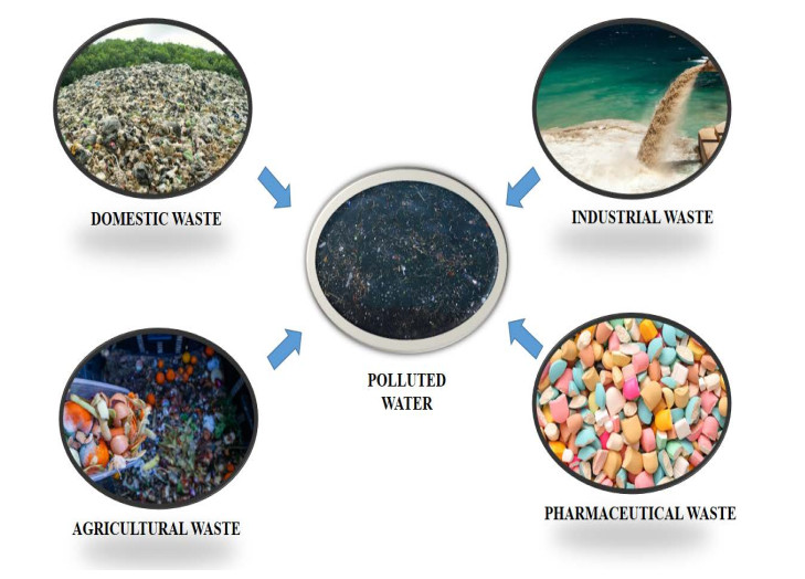
In this review, we describe recent developments and strategies involved in the utilization of solid supports for the management of wastewater by means of biological treatments. The origin of wastewater determines whether it is considered natural or industrial waste, and the source(s) singly or collectively contribute to increase water pollution. Pollution is a threat to aquatic and humans; thus, before the discharge of treated waters back into the environment, wastewater is put through a number of treatment processes to ensure its safety for human use. Biological treatment or bioremediation has become increasingly popular due to its positive impact on the ecosystem, high level of productivity, and process application cost-effectiveness. Bioremediation involving the use of microbial cell immobilization has demonstrated enhanced effectiveness compared to free cells. This constitutes a significant departure from traditional bioremediation practices (entrapment, adsorption, encapsulation), in addition to its ability to engage in covalent bonding and cross-linking. Thus, we took a comparative look at the existing and emerging immobilization methods and the related challenges, focusing on the future. Furthermore, our work stands out by highlighting emerging state-of-the-art tools that are bioinspired [enzymes, reactive permeable barriers linked to electrokinetic, magnetic cross-linked enzyme aggregates (CLEAs), bio-coated films, microbiocenosis], as well as the use of nanosized biochar and engineered cells or their bioproducts targeted at enhancing the removal efficiency of metals, carbonates, organic matter, and other toxicants and pollutants. The potential integration of 'omics' technologies for enhancing and revealing new insights into bioremediation via cell immobilization is also discussed.

| [1] |
Owa FD (2013) Water pollution:Sources, effects, control and management. Mediterranean J. Social Sci 4:66. https://doi.org/10.5901/mjss.2013.v4n8p65 doi: 10.5901/mjss.2013.v4n8p65

|
| [2] | Kumar RDH, Lee SM (2012) Water pollution and treatment technologies. J Environ Anal Toxicol 2: e103. https://doi.org/10.4172/2161-0525.1000e103 |
| [3] | Ministry of Environmental Protection, MEP releases the 2014 Report on the state of environment in China, 2014. Available from: https://english.mee.gov.cn/News_service/news_release/201506/t20150612_303436.shtml. |
| [4] | Miao Y, Fan C, Guo J (2012) China's water environmental problems and improvement measures. Environ Resour Econ 3:43-44. |
| [5] | World Bank Group, Pakistan - Strategic country environmental assessment, Main Report no. 36946-PK World Bank, 2006. Available from: http://documents.worldbank.org/curated/en/132221468087836074/Main-report |
| [6] |
Cutler DM, Miller G (2005) The role of public health improvements in health advances:The twentieth-century United States. Demography 42:1-22. https://doi.org/10.1353/dem.2005.0002 doi: 10.1353/dem.2005.0002
|
| [7] |
Jalan J, Ravallion M (2003) Does piped water reduce diarrhea for children in rural India? J Econ 112:153-173. https://doi.org/10.1016/S0304-4076(02)00158-6 doi: 10.1016/S0304-4076(02)00158-6
|
| [8] | Roushdy R, Sieverding M, Radwan H (2012) The impact of water supply and sanitation on child health: Evidence from Egypt. New York Population Council, New York, 1–72. Available from: https://doi.org/10.31899/pgy3.1016 |
| [9] |
Lu YL, Song S, Wang RS, et al. (2015) Impacts of soil and water pollution on food safety and health risks in China. Environ Int 77:5-15. https://doi.org/10.1016/j.envint.2014.12.010 doi: 10.1016/j.envint.2014.12.010
|
| [10] | Lin NF, Tang J, Ismael HSM (2000) Study on environmental etiology of high incidence areas of liver cancer in China. World J. Gastroenterol 6:572-576. |
| [11] |
Morales-Suarez-Varela MM, Llopis-Gonzalez A, Tejerizo-Perez ML (1995) Impact of nitrates in drinking water on cancer mortality in Valencia, Spain. Eur J Epidemiol 11:15-21. https://doi.org/10.1007/BF01719941 doi: 10.1007/BF01719941
|
| [12] |
Ebenstein A (2012) The consequences of industrialization:Evidence from water pollution and digestive cancers in China. Rev Econ Stats 94:186-201. https://doi.org/10.1162/REST_a_00150 doi: 10.1162/REST_a_00150
|
| [13] |
Teh CY, Budiman PM, Shak KPY, et al. (2016) Recent advancement of coagulation-flocculation and its application in wastewater treatment. Ind Eng Chem Res 55:4363-4389. https://doi.org/10.1021/acs.iecr.5b04703 doi: 10.1021/acs.iecr.5b04703
|
| [14] | Pontius FW (1990) Water quality and treatment. (4th Ed), New York: McGrawHill, Inc. |
| [15] | Xiaofan Z, Shaohong Y, Lili M, et al. (2015) The application of immobilized microorganism technology in wastewater treatment. 2nd International Conference on Machinery, Materials Engineering, Chemical Engineering and Biotechnology (MMECEB 2015). Pp. 103–106. |
| [16] | Malovanyy M, Masikevych A, Masikevych Y, et al. (2022) Use of microbiocenosis immobilized on carrier in technologies of biological treatment of surface and wastewater. J Ecol Eng 23:34-43.https: //doi.org/10.12911/22998993/151146 |
| [17] |
Wang L, Cheng WC, Xue ZF, et al. (2023) Study on Cu-and Pb-contaminated loess remediation using electrokinetic technology coupled with biological permeable reactive barrier. J Environ Manage 348:119348. https://doi.org/10.1016/j.jenvman.2023.119348 doi: 10.1016/j.jenvman.2023.119348
|
| [18] |
Wang L, Cheng WC, Xue ZF, et al. (2024) Struvite and ethylenediaminedisuccinic acid (EDDS) enhance electrokinetic-biological permeable reactive barrier removal of copper and lead from contaminated loess. J Environ Manage 360:121100. https://doi.org/10.1016/j.jenvman.2024.121100 doi: 10.1016/j.jenvman.2024.121100
|
| [19] |
Dombrovskiy KO, Rylskyy OF, Gvozdyak PI (2020) The periphyton structural organization on the fibrous carrier "viya" over the waste waters purification from the oil products. Hydrobiol J 56:87-96. https://doi.org/10.1615/HydrobJ.v56.i3.70 doi: 10.1615/HydrobJ.v56.i3.70
|
| [20] |
Zhang Y, Piao M, He L, (2020) Immobilization of laccase on magnetically separable biochar for highly efficient removal of bisphenol A in water. RSC Adv 10:4795-4804. https://doi.org/10.1039/C9RA08800H doi: 10.1039/C9RA08800H
|
| [21] |
Najim AA, Radeef AY, al-Doori I, et al. (2024) Immobilization:the promising technique to protect and increase the efficiency of microorganisms to remove contaminants. J Chem Technol Biotechnol 99:1707-1733. https://doi.org/10.1002/jctb.7638 doi: 10.1002/jctb.7638
|
| [22] |
Zhang K, Luo X, Yang L, et al. (2021) Progress toward hydrogels in removing heavy metals from water:Problems and solutions-A review. ACS ES&T Water 1:1098-1116. https://doi.org/10.1021/acsestwater.1c00001 doi: 10.1021/acsestwater.1c00001
|
| [23] | Olaniran NS (1995) Environment and health: An introduction, In Olaniran NS et al. (Eds) Environment and Health. Lagos, Nigeria: Macmillan, for NCF, 34–151. |
| [24] |
Singh G, Kumari B, Sinam G, (2018) Fluoride distribution and contamination in the water, soil and plants continuum and its remedial technologies, an Indian perspective-A review.Environ Poll239:95-108. https://doi.org/10.1016/j.envpol.2018.04.002 doi: 10.1016/j.envpol.2018.04.002
|
| [25] |
Schwarzenbach RP, Escher BI, Fenner K, (2006) The challenge of micropollutants in aquatic systems. Science 313:1072-1077. https://doi.org/10.1126/science.1127291 doi: 10.1126/science.1127291
|
| [26] |
Ma J, Ding Z, Wei G, et al. (2009) Sources of water pollution and evolution of water quality in the Wuwei basin of Shiyang river, Northwest China.J Environ Manage90:1168-1177. https://doi.org/10.1016/j.jenvman.2008.05.007 doi: 10.1016/j.jenvman.2008.05.007
|
| [27] | Abdulmumini A, Gumel SM, Jamil G (2015) Industrial effluents as major source of water pollution in Nigeria:An overview. Am J Chem Appl 1:45-50. |
| [28] | Fakayode O (2005) Impact assessment of industrial effluent on water quality of the receiving Alaro River in Ibadan. Nigerian Afr J Environ Assoc Manage 10:1-13 |
| [29] |
Begum A, Ramaiah M, Harikrishna, I, (2009) Heavy metals pollution and chemical profile of Cauvery of river water. J Chem 6:45-52. https://doi.org/10.1155/2009/154610 doi: 10.1155/2009/154610
|
| [30] | Sunita S, Darshan M, Jayita T, (2014) A comparative analysis of the physico-chemical properties and heavy metal pollution in three major rivers across India. Int J Sci Res 3:1936-1941. |
| [31] |
Li J, Yang Y, Huan H, et al. (2016) Method for screening prevention and control measures and technologies based on groundwater pollution intensity assessment. Sci Total Environ 551:143-154. https://doi.org/10.1016/j.scitotenv.2015.12.152 doi: 10.1016/j.scitotenv.2015.12.152
|
| [32] |
Yuanan H, Hefa C (2013) Water pollution during China's industrial transition. Environ Dev 8:57-73. https://doi.org/10.1016/j.envdev.2013.06.001 doi: 10.1016/j.envdev.2013.06.001
|
| [33] |
Li W, Hongbin W (2021) Control of urban river water pollution is studied based on SMS. Environ Technol Innov 22:101468. https://doi.org/10.1016/j.eti.2021.101468 doi: 10.1016/j.eti.2021.101468
|
| [34] | Swapnil MK (2014) Water pollution and public health issues in Kolhapur city in Maharashtra. Int J Sci Res Pub 4:1-6. |
| [35] |
Qijia C, Yong H, Hui W, (2019) Diversity and abundance of bacterial pathogens in urban rivers impacted by domestic sewage. Environ Pollut 249:24-35. https://doi.org/10.1016/j.envpol.2019.02.094 doi: 10.1016/j.envpol.2019.02.094
|
| [36] | Ministry of Environmental Protection (MEP), 2011 China State of the Environment. China Environmental Science Press, Beijing, China, 2012. |
| [37] |
Gao C, Zhang T (2010) Eutrophication in a Chinese context:Understanding various physical and socio-economic aspects. Ambio 39:385-393. https://doi.org/10.1007/s13280-010-0040-5 doi: 10.1007/s13280-010-0040-5
|
| [38] | Chanti BP, Prasadu DK (2015) Impact of pharmaceutical wastes on human life and environment. RCJ 8:67-70. |
| [39] | World Health Organization, WHO (2013) Water sanitation and health. Available from: https://www.who.int/teams/environment-climate-change-and-health/water-sanitation-and-health |
| [40] | Sayadi MH, Trivedy RK, Pathak RK (2010) Pollution of pharmaceuticals in environment. J Ind Pollut Control |
| [41] |
Fick J, Söderström H, Lindberg RH, (2009) Contamination of surface, ground, and drinking water from pharmaceutical production. Environ Toxicol Chem 28:2522-2527. https://doi.org/10.1897/09-073.1 doi: 10.1897/09-073.1
|
| [42] | Rosen M, Welander T, Lofqvist A (1998) Development of a new process for treatment of a pharmaceutical wastewater. Water Sci Technol 37:251-258. |
| [43] | Niraj ST, Attar SJ, Mosleh MM (2011) Sewage/wastewater treatment technologies. Sci Revs Chem Commun 1:18-24 |
| [44] |
Martins SCS, Martins CM, Oliveira, Fiúza LMCG, (2013) Immobilization of microbial cells:A promising tool for treatment of toxic pollutants in industrial wastewater. Afr J Biotechnol 12:4412-4418. https://doi.org/10.5897/AJB12.2677 doi: 10.5897/AJB12.2677
|
| [45] |
Cassidy MB, Lee H, Trevors JT (1996) Environmental applications of immobilized microbial cells:A review. J Ind Microbiol 16:79-101. https://doi.org/10.1007/BF01570068 doi: 10.1007/BF01570068
|
| [46] |
Wada M, Kato J, Chibata I (1979) A new immobilization of microbial cells. Appl Microbiol Biotechnol 8:241-247. https://doi.org/10.1007/BF00508788 doi: 10.1007/BF00508788
|
| [47] |
Park JK, Chang HN (2000) Microencapsulation of microbial cells. Biotechnol Adv 18:303-319. https://doi.org/10.1016/S0734-9750(00)00040-9 doi: 10.1016/S0734-9750(00)00040-9
|
| [48] |
Mrudula S, Shyam N (2012) Immobilization of Bacillus megaterium MTCC 2444 by Ca-alginate entrapment method for enhanced alkaline protease production. Braz Arch Biol Technol 55:135-144. https://doi.org/10.1590/S1516-89132012000100017 doi: 10.1590/S1516-89132012000100017
|
| [49] | Xia B, Zhao Q, Qu Y (2010) The research of different immobilized microorganisms' technologies and carriers in sewage disposal. Sci Technol Inf 1:698-699. |
| [50] |
Han M, Zhang C, Ho SH (2023) Immobilized microalgal system:An achievable idea for upgrading current microalgal wastewater treatment. ESE 1:100227. https://doi.org/10.1016/j.ese.2022.100227 doi: 10.1016/j.ese.2022.100227
|
| [51] |
Wang Z, Ishii S, Novak PJ (2021) Encapsulating microorganisms to enhance biological nitrogen removal in wastewater:recent advancements and future opportunities. Environ Sci:Water Sci Technol 7:1402-1416. https://doi.org/10.1039/D1EW00255D doi: 10.1039/D1EW00255D
|
| [52] |
Tong CY, Derek CJ (2023) Bio-coatings as immobilized microalgae cultivation enhancement:A review. Sci Total Environ 20:163857. https://doi.org/10.1016/j.scitotenv.2023.163857 doi: 10.1016/j.scitotenv.2023.163857
|
| [53] |
Dzionek A, Wojcieszyńska D, Guzik U (2022) Use of xanthan gum for whole cell immobilization and its impact in bioremediation-a review. Bioresour Technol 351:126918. https://doi.org/10.1016/j.biortech.2022.126918 doi: 10.1016/j.biortech.2022.126918
|
| [54] | Blanco A, Sampedro MA, Sanz B, et al. (2023) Immobilization of non-viable cyanobacteria and their use for heavy metal adsorption from water. In Environmental biotechnology and cleaner bioprocesses, CRC Press, 2023,135–153. https://doi.org/10.1201/9781003417163-14 |
| [55] |
Saini S, Tewari S, Dwivedi J, et al. (2023) Biofilm-mediated wastewater treatment:a comprehensive review. Mater Adv 4:1415-1443. https://doi.org/10.1039/D2MA00945E doi: 10.1039/D2MA00945E
|
| [56] |
Bouabidi ZB, El-Naas MH, Zhang Z (2019) Immobilization of microbial cells for the biotreatment of wastewater:A review. Environ Chem Lett 17:241-257. https://doi.org/10.1007/s10311-018-0795-7 doi: 10.1007/s10311-018-0795-7
|
| [57] |
Fortman DJ, Brutman JP, De Hoe GX, et al. (2018) Approaches to sustainable and continually recyclable cross-linked polymers. ACS Sustain Chem Eng 6:11145-11159. https://doi.org/10.1021/acssuschemeng.8b02355 doi: 10.1021/acssuschemeng.8b02355
|
| [58] |
Mahmoudi C, Tahraoui DN, Mahmoudi H, et al. (2024) Hydrogels based on proteins cross-linked with carbonyl derivatives of polysaccharides, with biomedical applications. Int J Mol Sci 25:7839. https://doi.org/10.3390/ijms25147839 doi: 10.3390/ijms25147839
|
| [59] | Waheed A, Mazumder MAJ, Al-Ahmed A, et al. (2019) Cell encapsulation. In Jafar MM, Sheardown H, Al-Ahmed A (Eds), Functional biopolymers, Polymers and polymeric composites: A reference series. Springer, Cham. https://doi.org/10.1007/978-3-319-95990-0_4 |
| [60] |
Chen S, Arnold WA, Novak PJ (2021) Encapsulation technology to improve biological resource recovery:recent advancements and research opportunities. Environ Sci Water Res Technol 7:16-23. https://doi.org/10.1039/D0EW00750A doi: 10.1039/D0EW00750A
|
| [61] | Tripathi A, Melo JS (2021) Immobilization Strategies:Biomedical, Bioengineering and Environmental Applications (Gels Horizons:From Science to Smart Materials), 676. https://doi.org/10.1007/978-981-15-7998-1p |
| [62] | Górecka E, Jastrzębska M (2011) Immobilization techniques and biopolymer carriers. Biotechnol Food Sci 75:65-86. |
| [63] |
Lopez A, Lazaro N, Marques AM (1997) The interphase technique:a simple method of cell immobilization in gel-beads. J of Microbiol Methods 30:231-234. https://doi.org/10.1016/S0167-7012(97)00071-7 doi: 10.1016/S0167-7012(97)00071-7
|
| [64] | Ramakrishna SV, Prakasha RS (1999) Microbial fermentations with immobilized cells. Curr Sci 77:87-100. |
| [65] |
Saberi RR, Skorik YA, Thakur VK, et al. (2021) Encapsulation of plant biocontrol bacteria with alginate as a main polymer material. Int J Mol Sci 22:11165. https://doi.org/10.3390/ijms222011165 doi: 10.3390/ijms222011165
|
| [66] |
Mohidem NA, Mohamad M, Rashid MU, et al. (2023) Recent advances in enzyme immobilisation strategies:An overview of techniques and composite carriers.J Compos Sci7:488. https://doi.org/10.3390/jcs7120488 doi: 10.3390/jcs7120488
|
| [67] |
Thomas D, O'Brien T, Pandit A (2018) Toward customized extracellular niche engineering:progress in cell-entrapment technologies. Adv Mater 30:1703948. https://doi.org/10.1002/adma.201703948 doi: 10.1002/adma.201703948
|
| [68] |
Farasat A, Sefti MV, Sadeghnejad S, et al. (2017) Mechanical entrapment analysis of enhanced preformed particle gels (PPGs) in mature reservoirs.J Pet Sci Eng157:441-450. https://doi.org/10.1016/j.petrol.2017.07.028 doi: 10.1016/j.petrol.2017.07.028
|
| [69] |
Sampaio CS, Angelotti JA, Fernandez-Lafuente R, et al. (2022) Lipase immobilization via cross-linked enzyme aggregates:Problems and prospects-A review. Int J Biol Macromol 215:434-449. https://doi.org/10.1016/j.ijbiomac.2022.06.139 doi: 10.1016/j.ijbiomac.2022.06.139
|
| [70] |
Picos-Corrales LA, Morales-Burgos AM, Ruelas-Leyva JP, et al. (2023) Chitosan as an outstanding polysaccharide improving health-commodities of humans and environmental protection.Polymers 15:526. https://doi.org/10.3390/polym15030526 doi: 10.3390/polym15030526
|
| [71] |
Gill J, Orsat V, Kermasha S (2018) Optimization of encapsulation of a microbial laccase enzymatic extract using selected matrices. Process Biochem 65:55-61. https://doi.org/10.1016/j.procbio.2017.11.011 doi: 10.1016/j.procbio.2017.11.011
|
| [72] |
Navarro JM, Durand G (1977) Modification of yeast metabolism by immobilization onto porous glass. Eur J Appl Microbiol 4:243-254. https://doi.org/10.1007/BF00931261 doi: 10.1007/BF00931261
|
| [73] |
Alkayyali T, Cameron T, Haltli B, et al. (2019) Microfluidic and cross-linking methods for encapsulation of living cells and bacteria-A review. Analytica Chimica Acta 1053:1-21. https://doi.org/10.1016/j.aca.2018.12.056 doi: 10.1016/j.aca.2018.12.056
|
| [74] |
Guisan JM, Fernandez-Lorente G, Rocha-Martin J, et al. (2022) Enzyme immobilization strategies for the design of robust and efficient biocatalysts. CRGSC 35:100593. https://doi.org/10.1016/j.cogsc.2022.100593 doi: 10.1016/j.cogsc.2022.100593
|
| [75] |
Qi F, Jia Y, Mu R, et al. (2021) Convergent community structure of algal bacterial consortia and its effect on advanced wastewater treatment and biomass production. Sci Rep 11:21118. https://doi.org/10.1038/s41598-021-00517-x doi: 10.1038/s41598-021-00517-x
|
| [76] |
Sharma M, Agarwal S, Agarwal MR, et al. (2023) Recent advances in microbial engineering approaches for wastewater treatment:a review. Bioengineered 14:2184518. https://doi.org/10.1080/21655979.2023.2184518 doi: 10.1080/21655979.2023.2184518
|
| [77] |
Cortez S, Nicolau A, Flickinger MC, et al. (2017) Biocoatings:A new challenge for environmental biotechnology. Biochem Eng J 121:25-37. https://doi.org/10.1016/j.bej.2017.01.004 doi: 10.1016/j.bej.2017.01.004
|
| [78] | Zhao LL, Pan B, Zhang W, et al. (2011) Polymer-supported nanocomposites for environmental application:a review Chem. Eng. J., 170:381-394. https://doi.org/10.1016/j.cej.2011.02.071 |
| [79] |
Flickinger MC, Schottel JL, Bond DR (2007) Scriven Painting and printing living bacteria:Engineering nanoporous biocatalytic coatings to preserve microbial viability and intensify reactivity. Biotechnol Prog 23:2-17. https://doi.org/10.1021/bp060347r doi: 10.1021/bp060347r
|
| [80] |
Martynenko NN, Gracheva IM, Sarishvili NG, et al. (2004) Immobilization of champagne yeasts by inclusion into cryogels of polyvinyl alcohol:Means of preventing cell release from the carrier matrix. Appl Biochem Microbiol 40:158-164. https://doi.org/10.1023/B:ABIM.0000018919.13036.19 doi: 10.1023/B:ABIM.0000018919.13036.19
|
| [81] |
Yang D, Shu-Qian F, Yu S, et al. (2015) A novel biocarrier fabricated using 3D printing technique for wastewater treatment. Sci Rep 5:12400. https://doi.org/10.1038/srep12400 doi: 10.1038/srep12400
|
| [82] |
Ayilara MS, Babalola OO (2023) Bioremediation of environmental wastes:the role of microorganisms. Front Agron 5:1183691. https://doi.org/10.3389/fagro.2023.1183691 doi: 10.3389/fagro.2023.1183691
|
| [83] | Kumar V, Garg VK, Kumar S, et al. (2022) Omics for environmental engineering and microbiology systems (Florida:CRC Press). https://doi.org/10.1201/9781003247883 |
| [84] |
Liu L, Wu Q, Miao X, et al. (2022) Study on toxicity effects of environmental pollutants based on metabolomics:A review. Chemosphere 286:131815. https://doi.org/10.1016/j.chemosphere.2021.131815 doi: 10.1016/j.chemosphere.2021.131815
|
| [85] |
Zdarta J, Jankowska K, Bachosz K, et al. (2021) Enhanced wastewater treatment by immobilized enzymes. Current Pollution Reports 7:167-179. https://doi.org/10.1007/s40726-021-00183-7 doi: 10.1007/s40726-021-00183-7
|
| [86] | Freeman A, Lilly MD (1998) Effect of processing parameters on the feasibility and operational stability of immobilized viable microbial cells. Enzyme Microb Technol 23 335-345. https://doi.org/10.1016/S0141-0229(98)00046-5 |
| [87] | Ligler FS, Taitt CR (2011) Optical biosensors: Today and tomorrow, Elsevier, Pp. 151. |
| [88] |
Ismail E, José D, Gonçalves V, et al. (2015) Principles, techniques, and applications of biocatalyst immobilization for industrial application. Appl Microbiol Biotechnol 99:2065-2082. https://doi.org/10.1007/s00253-015-6390-y doi: 10.1007/s00253-015-6390-y
|
| [89] |
Anselmo AM, Novais JM (1992) Degradation of phenol by immobilized mycelium of Fusarium flocciferum in continuous culture. Water Sci Technol 25:161-168.https://doi.org/10.2166/wst.1992.0024 doi: 10.2166/wst.1992.0024
|
| [90] | Liu Z, Yang H, Jia S (1992) Study on decolorization of dyeing wastewater by mixed bacterial cells immobilized in polyvinyl alcohol (PVA). China Environ Sci 13:2-6. |
| [91] | Guomin C, Zhao Q, Gong J (2001) Study on nitrogen removal from wastewater in a new co-immobilized cells membrane bioreactor. Acta Sci Circumst. 21:189-193. |
| [92] | Jogdand VG, Chavan PA, Ghogare PD, et al. (2012) Remediation of textile industry waste-water using immobilized Aspergillus terreus. Eur J Exp Biol 2:1550-1555 |
| [93] |
Adlercreutz P, Holst O, Mattiasson B (1982) Oxygen supply to immobilized cells:2. Studies on a coimmobilized algae-bacteria preparation with in situ oxygen generation. Enzyme Microb Tech 4:395-400. https://doi.org/10.1016/0141-0229(82)90069-2 doi: 10.1016/0141-0229(82)90069-2
|
| [94] |
Chevalier P, de la Noüe J (1988) Behavior of algae and bacteria co-immobilized in carrageenan, in a fluidized bed. Enzyme Microb Tech 10:19-23. https://doi.org/10.1016/0141-0229(88)90093-2 doi: 10.1016/0141-0229(88)90093-2
|
| [95] |
Wikström P, Szwajcer E, Brodelius P, et al. (1982) Formation of α-keto acids from amino acids using immobilized bacteria and algae. Biotechnol Lett 4:153-158. https://doi.org/10.1007/BF00144316 doi: 10.1007/BF00144316
|
| [96] |
Serebrennikova MK, Golovina EE, Kuyukina MS, et al. (2017) A consortium of immobilized Rhodococci for oil field wastewater treatment in a column bioreactor. Appl Biochem Microbiol 53:435-440. https://doi.org/10.1134/S0003683817040123 doi: 10.1134/S0003683817040123
|
| [97] |
Choi M, Chaudhary R, Lee M, et al. (2020) Enhanced selective enrichment of partial nitritation and anammox bacteria in a novel two-stage continuous flow system using flat-type poly(vinylalcohol) cryogel films. Bioresour Technol 300:122546. https://doi.org/10.1016/j.biortech.2019.122546 doi: 10.1016/j.biortech.2019.122546
|
| [98] |
Yordanova G, Ivanova D, Godjevargova T, et al. (2009) Biodegradation of phenol by immobilized Aspergillus awamori NRRL 3112 on modified polyacrylonitrile membrane. Biodegradation 20:717-726. https://doi.org/10.1007/s10532-009-9259-x doi: 10.1007/s10532-009-9259-x
|
| [99] | Tekere M (2019) Microbial bioremediation and different bioreactors designs applied. In Biotechnology and Bioengineering; IntechOpen: London, UK, Pp. 1–19. https://doi.org/10.5772/intechopen.83661 |
| [100] |
Liu SH, Zeng ZT, Niu QY, et al. (2019) Influence of immobilization on phenanthrene degradation by Bacillus sp. P1 in the presence of Cd (II). Sci Total Environ 655:1279-1287. https://doi.org/10.1016/j.scitotenv.2018.11.272 doi: 10.1016/j.scitotenv.2018.11.272
|
| [101] |
Liu SH, Lin HH, Lai CY, et al. (2019) Microbial community in a pilot-scale biotrickling filter with cell-immobilized biochar beads and its performance in treating toluene-contaminated waste gases. Int Biodeterior Biodegrad 144:104743. https://doi.org/10.1016/j.ibiod.2019.104743 doi: 10.1016/j.ibiod.2019.104743
|
| [102] |
Önnby L, Pakade V, Mattiasson B, et al. (2012) Polymer composite adsorbents using particles of molecularly imprinted polymers or aluminium oxide nanoparticles for treatment of arsenic contaminated waters. Water Res 46:4111-4120. https://doi.org/10.1016/j.watres.2012.05.028 doi: 10.1016/j.watres.2012.05.028
|
| [103] |
Baimenov A, Berillo D, Azat S, et al. (2020) Removal of Cd2+ from water by use of super-macroporous cryogels and comparison to commercial adsorbents. Polymers 12:2405. https://doi.org/10.3390/polym12102405 doi: 10.3390/polym12102405
|
| [104] |
Baimenov AZ, Berillo DA, Moustakas K, et al. (2020) Efficient removal of mercury (II) from water by use of cryogels and comparison to commercial adsorbents under environmentally relevant conditions. J Hazard Mater 399:123056. https://doi.org/10.1016/j.jhazmat.2020.123056 doi: 10.1016/j.jhazmat.2020.123056
|
| [105] |
Safonova E, Kvitko KV, Iankevitch MI, et al. (2004) Biotreatment of industrial wastewater by selected algal-bacterial consortia. Eng Life Sci 4:347-353. https://doi.org/10.1002/elsc.200420039 doi: 10.1002/elsc.200420039
|
| [106] |
Blanco A, Sanz B, Llama MJ, et al. (1999) Biosorption of heavy metals to immobilized Phormidium laminosum biomass. J Biotechnol 69:227-240. https://doi.org/10.1016/S0168-1656(99)00046-2 doi: 10.1016/S0168-1656(99)00046-2
|
| [107] |
Somerville HJ, Mason JR, Ruffell RN (1977) Benzene degradation by bacterial cells immobilized in polyacrylamide gel. Appl Microbiol Biotechnol 4:75-85. https://doi.org/10.1007/BF00929158 doi: 10.1007/BF00929158
|
| [108] |
Tsai SL, Lin CW, Wu CH, et al. (2013) Kinetics of xenobiotic biodegradation by the Pseudomonas sp. YATO411 strain in suspension and cell-immobilized beads. J Taiwan Inst Chem Eng 44:303-309. https://doi.org/10.1016/j.jtice.2012.11.004 doi: 10.1016/j.jtice.2012.11.004
|
| [109] |
Akhtar N, Saeed A, Iqbal M (2003) Chlorella sorokiniana immobilized on the biomatrix of vegetable sponge of Luffa cylindrica:a new system to remove cadmium from contaminated aqueous medium. Bioresour Technol 88:163-165. https://doi.org/10.1016/S0960-8524(02)00289-4 doi: 10.1016/S0960-8524(02)00289-4
|
| [110] |
Saeed A, Iqbal M (2006) Immobilization of blue green microalgae on loofa sponge to biosorb cadmium in repeated shake flask batch and continuous flow fixed bed column reactor system. World J Microb Biotechnol 22:775-782. https://doi.org/10.1007/s11274-005-9103-3 doi: 10.1007/s11274-005-9103-3
|
| [111] |
Rangasayatorn N, Pokethitiyook P, Upatahm ES, et al. (2004) Cadmium biosorption by cells of Spirulina platensis TISTR 8217 immobilized in alginate and silica gel. Environ Int 30:57-63. https://doi.org/10.1016/S0160-4120(03)00146-6 doi: 10.1016/S0160-4120(03)00146-6
|
| [112] | Mohamed AA, Ahmed MA, Mahmoud ME, et al. (2019) Bioremediation of a pesticide and selected heavy metals in wastewater from various sources using a consortium of microalgae and cyanobacteria. Slov Vet Res 56:61-74. |
| [113] |
Aslıyüce S, Denizli A (2017) Design of PHEMA Cryogel as Bioreactor Matrices for Biological Cyanide Degradation from Waste-water. Hacet J Biol Chem 45:639-645. https://doi.org/10.15671/HJBC.2018.208 doi: 10.15671/HJBC.2018.208
|
| [114] |
Suner SS, Sahiner N (2018) Humic acid particle embedded super porous gum Arabic cryogel network for versatile use. Polym Adv Technol 29:151-159. https://doi.org/10.1002/pat.4097 doi: 10.1002/pat.4097
|
| [115] | Sharma A, Bhat S, Vishnoi T, et al. (2013). Three-dimensional super macroporous carrageenan-gelatin cryogel matrix for tissue engineering applications. BioMed Res Int 2013: 478279. |
| [116] |
Le Noir M, Plieva FM, Mattiasson B (2009) Removal of endocrine-disrupting compounds from water using macroporous molecularly imprinted cryogels in a moving-bed reactor. J Sep Sci 32:1471-1479. https://doi.org/10.1002/jssc.200800670 doi: 10.1002/jssc.200800670
|
| [117] |
See S, Lim PE, Lim JW, et al. (2005) Evaluation of o-cresol removal using PVA-cryogel-immobilised biomass enhanced by PAC. Water SA 41:55-60. https://doi.org/10.4314/wsa.v41i1.8 doi: 10.4314/wsa.v41i1.8
|
| [118] |
Gao S, Wang Y, Diao X, et al. (2010) Effect of pore diameter and cross-linking method on the immobilization efficiency of Candida rugose lipase in SBA-15. Bioresour Technol 101:3830-3837. https://doi.org/10.1016/j.biortech.2010.01.023 doi: 10.1016/j.biortech.2010.01.023
|
| [119] |
Stepanov N, Efremenko E (2018) Deceived concentrated immobilized cells as biocatalyst for intensive bacterial cellulose production from various sources. Catalysts 8:33. https://doi.org/10.3390/catal8010033 doi: 10.3390/catal8010033
|
| [120] |
Zaushitsyna O, Berillo D, Kirsebom H, et al. (2014) Cryostructured and crosslinked viable cells forming monoliths suitable for bioreactor applications. Top Catal 57:339-348. https://doi.org/10.1007/s11244-013-0189-9 doi: 10.1007/s11244-013-0189-9
|
| [121] |
Qian L, Zhang H (2011) Controlled freezing and freeze drying:A versatile route for porous and micro-/nano-structured materials. J Chem Technol Biotechnol 86:172-184. https://doi.org/10.1002/jctb.2495 doi: 10.1002/jctb.2495
|

Figures(2) / Tables(3)

Frank Abimbola Ogundolie, Olorunfemi Oyewole Babalola, Charles Oluwaseun Adetunji, Christiana Eleojo Aruwa, Jacqueline Njikam Manjia, Taoheed Kolawole Muftaudeen. A review on bioremediation by microbial immobilization-an effective alternative for wastewater treatment[J]. AIMS Environmental Science, 2024, 11(6): 918-939. doi: 10.3934/environsci.2024046


 DownLoad: