This paper presented a comprehensive study of a three-dimensional nonlinear system of difference equations, which can be reduced to a two-dimensional bilinear system. The system monitored the evolution of three sequences $ \left(P_{m}\right), $ $ \left(Q_{m}\right), $ $ \left(R_{m}\right) $, governed by recursive relations. We investigated the solvability of this system and provided general closed-form solutions for various parameter conditions. Furthermore, the simulations provided valuable insights into the dynamic behavior of animals, modeled using recursive difference equations. The model encapsulated essential behavioral metrics, represented by the variables $ P $, $ Q $, and $ R $, which corresponded to individual actions, social interactions, and environmental stressors, respectively. These variables adapted dynamically in response to internal and external influences, illustrating the system's sensitivity to various behavioral and environmental conditions.
Citation: Hashem Althagafi, Ahmed Ghezal. Solving a system of nonlinear difference equations with bilinear dynamics[J]. AIMS Mathematics, 2024, 9(12): 34067-34089. doi: 10.3934/math.20241624
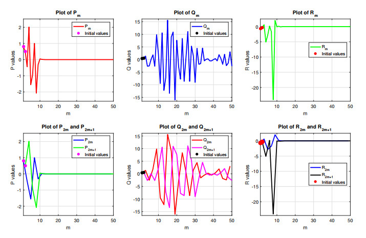
This paper presented a comprehensive study of a three-dimensional nonlinear system of difference equations, which can be reduced to a two-dimensional bilinear system. The system monitored the evolution of three sequences $ \left(P_{m}\right), $ $ \left(Q_{m}\right), $ $ \left(R_{m}\right) $, governed by recursive relations. We investigated the solvability of this system and provided general closed-form solutions for various parameter conditions. Furthermore, the simulations provided valuable insights into the dynamic behavior of animals, modeled using recursive difference equations. The model encapsulated essential behavioral metrics, represented by the variables $ P $, $ Q $, and $ R $, which corresponded to individual actions, social interactions, and environmental stressors, respectively. These variables adapted dynamically in response to internal and external influences, illustrating the system's sensitivity to various behavioral and environmental conditions.

| [1] |
A. Ghezal, O. Alzeley, Probabilistic properties and estimation methods for periodic threshold autoregressive stochastic volatility, AIMS Math., 9 (2024), 11805–11832. https://doi.org/10.3934/math.2024578 doi: 10.3934/math.2024578

|
| [2] |
A. Ghezal, M. Balegh, I. Zemmouri, Markov-switching threshold stochastic volatility models with regime changes, AIMS Math., 9 (2024), 3895–3910. https://doi.org/10.3934/math.2024192 doi: 10.3934/math.2024192
|
| [3] | A. D. Moivre, Miscellanea analytica de seriebus et quadraturis, J. Tonson and J. Watts, Londini, 1730. |
| [4] | J. L. Lagrange, Sur l'intégration d'une équation différentielle à différences finies, qui contient la théorie des suites récurrentes, Miscellanea Taurinensia, 1759, 33–42. |
| [5] | G. Boole, A treatsie on the calculus of finite differences, 3 Eds., London: Macmillan and Co., 1880. |
| [6] | H. Levy, F. Lessman, Finite difference equations, New York: The Macmillan Company, 1961. |
| [7] | C. Jordan, Calculus of finite differences, New York: Chelsea Publishing Company, 1965. |
| [8] |
R. A. Zeid, Global behavior of two third order rational difference equations with quadratic terms, Math. Slovaca, 69 (2019), 147–158. http://dx.doi.org/10.1515/ms-2017-0210 doi: 10.1515/ms-2017-0210
|
| [9] |
R. A. Zeid, C. Cinar, Global behavior of the difference equation $x_{n+1} = \left. Ax_{n-1}\right/ B-Cx_{n}x_{n-2}$, Bol. Soc. Parana. Mat., 31 (2013), 43–49. http://dx.doi.org/10.5269/bspm.v31i1.14432 doi: 10.5269/bspm.v31i1.14432
|
| [10] |
I. M. Alsulami, E. M. Elsayed, On a class of nonlinear rational systems of difference equations, AIMS Math., 8 (2023), 15466–15485. https://doi.org/10.3934/math.2023789 doi: 10.3934/math.2023789
|
| [11] |
M. Gümüş, R. A. Zeid, Global behavior of a rational second order difference equation, J. Appl. Math. Comput., 62 (2020), 119–133. https://doi.org/10.1007/s12190-019-01276-9 doi: 10.1007/s12190-019-01276-9
|
| [12] |
N. Attia, A. Ghezal, Global stability and co-balancing numbers in a system of rational difference equations, Electron. Res. Arch., 32 (2024), 2137–2159. https://doi.org/10.3934/era.2024097 doi: 10.3934/era.2024097
|
| [13] |
H. Althagafi, A. Ghezal, Analytical study of nonlinear systems of higher-order difference equations: Solutions, stability, and numerical simulations, Mathematics, 12 (2024), 1159. https://doi.org/10.3390/math12081159 doi: 10.3390/math12081159
|
| [14] |
M. Kara, Investigation of the global dynamics of two exponential-form difference equations systems, Electron. Res. Arch., 31 (2023), 6697–6724. https://doi.org/10.3934/era.2023338 doi: 10.3934/era.2023338
|
| [15] |
C. Schinas, Invariants for difference equations and systems of difference equations of rational form, J. Math. Anal. Appl., 216 (1997), 164–179. https://doi.org/10.1006/jmaa.1997.5667 doi: 10.1006/jmaa.1997.5667
|
| [16] |
S. Stević, On the system of difference equations $x_{n} = c_{n}y_{n-3}/(a_{n}+b_{n}y_{n-1}x_{n-2}y_{n-3})$, $y_{n} = \gamma _{n}x_{n-3}/(\alpha_{n}+\beta_{n}x_{n-1}y_{n-2}x_{n-3})$, Appl. Math. Comput., 219 (2013), 4755–4764. https://doi.org/10.1016/j.amc.2012.10.092 doi: 10.1016/j.amc.2012.10.092
|
| [17] |
S. Stević, J. Diblik, B. Iri$ \overset{˘}{\mathop{\text{c}}} $anin, Z. $ \overset{˘}{\mathop{\text{S}}} $marda, On a third-order system of difference equations with variable coefficients, Abstr. Appl. Anal., 2012. https://doi.org/10.1155/2012/508523 doi: 10.1155/2012/508523
|
| [18] |
S. Stević, D. T. Tollu, On a two-dimensional nonlinear system of difference equations close to the bilinear system, AIMS Math., 8 (2023), 20561–20575. https://doi.org/10.3934/math.20231048 doi: 10.3934/math.20231048
|
| [19] |
X. Yang, W. Qiu, H. Chen, H. Zhang, Second-order BDF ADI Galerkin finite element method for the evolutionary equation with a nonlocal term in three-dimensional space, Appl. Numer. Math., 172 (2022), 497–513. https://doi.org/10.1016/j.apnum.2021.11.004 doi: 10.1016/j.apnum.2021.11.004
|
| [20] |
X. Yang, Z. Zhang, Superconvergence analysis of a robust orthogonal gauss collocation method for 2D fourth-order subdiffusion equations, J. Sci. Comput., 100 (2024), 62. https://doi.org/10.1007/s10915-024-02616-z doi: 10.1007/s10915-024-02616-z
|
| [21] |
X. Yang, Z. Zhang, Analysis of a new NFV scheme preserving DMP for two-dimensional sub-diffusion equation on distorted meshes, J. Sci. Comput., 99 (2024), 80. https://doi.org/10.1007/s10915-024-02511-7 doi: 10.1007/s10915-024-02511-7
|


Figures(13)

Hashem Althagafi, Ahmed Ghezal. Solving a system of nonlinear difference equations with bilinear dynamics[J]. AIMS Mathematics, 2024, 9(12): 34067-34089. doi: 10.3934/math.20241624


 DownLoad: