Threshold dynamics of stochastic SIRSW infectious disease model with multiparameter perturbation

Zhengwen Yin; Yuanshun Tan; Zhengwen Yin; Yuanshun Tan

doi:10.3934/math.20241597

AIMS Mathematics

2024, Volume 9, Issue 12: 33467-33492. doi: 10.3934/math.20241597

Previous Article Next Article

Research article

Threshold dynamics of stochastic SIRSW infectious disease model with multiparameter perturbation

Zhengwen Yin ,
Yuanshun Tan ^,

College of Mathematics and Statistics, Chongqing Jiaotong University, Chongqing 400074, China

Received: 22 September 2024 Revised: 06 November 2024 Accepted: 18 November 2024 Published: 25 November 2024
MSC : 34F05, 60G10

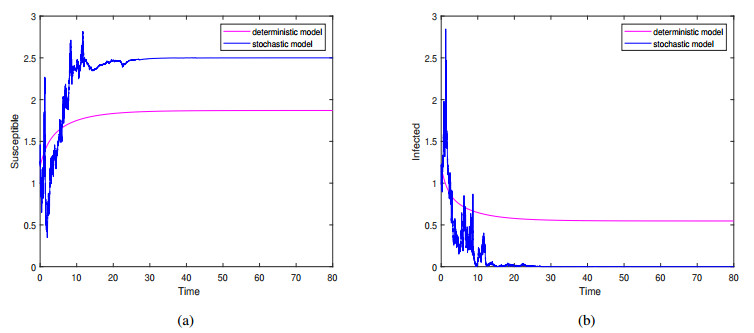
In this paper, we investigated a stochastic SIRS epidemic infectious disease model that accounted for environmentally driven infection and incorporated multiparameter perturbations. In addition to establishing the existence and uniqueness of the global positive solution of the model, we derived the threshold conditions for the extinction and persistence of the disease using the comparison theorem and It$ \hat{o} $'s formula of stochastic differential equations. Subsequently, we obtained the asymptotic stability of both the disease-free equilibrium and the endemic equilibrium of the deterministic model corresponding to the stochastic model through stochastic stability theory. The results indicated that high-intensity noise perturbation can inhibit the spread of the disease, and the dynamic behavior of the disease transitioned from persistence to extinction as noise intensity increased. Our study also demonstrated that, compared to perturbations in the indirect infection rate, changes in noise intensity that affect the direct infection rate will have a more significant impact on disease transmission.
- SIRS epidemic model,
- environmental driven infections,
- threshold dynamics,
- multiparameter perturbation
Citation: Zhengwen Yin, Yuanshun Tan. Threshold dynamics of stochastic SIRSW infectious disease model with multiparameter perturbation[J]. AIMS Mathematics, 2024, 9(12): 33467-33492. doi: 10.3934/math.20241597

Related Papers:

Abstract

In this paper, we investigated a stochastic SIRS epidemic infectious disease model that accounted for environmentally driven infection and incorporated multiparameter perturbations. In addition to establishing the existence and uniqueness of the global positive solution of the model, we derived the threshold conditions for the extinction and persistence of the disease using the comparison theorem and It$ \hat{o} $'s formula of stochastic differential equations. Subsequently, we obtained the asymptotic stability of both the disease-free equilibrium and the endemic equilibrium of the deterministic model corresponding to the stochastic model through stochastic stability theory. The results indicated that high-intensity noise perturbation can inhibit the spread of the disease, and the dynamic behavior of the disease transitioned from persistence to extinction as noise intensity increased. Our study also demonstrated that, compared to perturbations in the indirect infection rate, changes in noise intensity that affect the direct infection rate will have a more significant impact on disease transmission.

References

[1]	W. O. Kermack, A. G. McKendrick, Contributions to the mathematical theory of epidemics–I, Bull. Math. Biol., 53 (1991), 33–55. https://doi.org/10.1007/BF02464423 doi: 10.1007/BF02464423
[2]	W. M. Liu, H. W. Hethcote, S. A. Levin, Dynamical behavior of epidemiological models with nonlinear incidence rates, J. Math. Biol., 25 (1987), 359–380. https://doi.org/10.1007/BF00277162 doi: 10.1007/BF00277162
[3]	H. C. Tuckwell, R. J. Williams, Some properties of a simple stochastic epidemic model of SIR type, Math. Biosci., 208 (2007), 76–97. https://doi.org/10.1016/j.mbs.2006.09.018 doi: 10.1016/j.mbs.2006.09.018
[4]	X. Wei, Global analysis of a network-based SIR epidemic model with a saturated treatment function, Int. J. Biomath., 17 (2024), 2350112. https://doi.org/10.1142/S1793524523501127 doi: 10.1142/S1793524523501127
[5]	J. Li, J. Zhang, Z. Ma, Global analysis of some epidemic models with general contact rate and constant immigration, Appl. Math. Mech., 25 (2004), 396–404. https://doi.org/10.1007/BF02437523 doi: 10.1007/BF02437523
[6]	C. Y. Ji, D. Q. Jiang, The extinction and persistence of a stochastic SIR model, Adv. Differ. Equations, 2017 (2017), 30. https://doi.org/10.1186/s13662-016-1068-z doi: 10.1186/s13662-016-1068-z
[7]	N. Wang, L. Zhang, Z. D. Teng, Dynamics in a reaction-diffusion epidemic model via environmental driven infection in heterogenous space, J. Biol. Dyn., 16 (2021), 373–396. https://doi.org/10.1080/17513758.2021.1900428 doi: 10.1080/17513758.2021.1900428
[8]	L. Liu, X. Q. Zhao, Y. Zhou, A tuberculosis model with seasonality, Bull. Math. Biol., 72 (2010), 931–952. https://doi.org/10.1007/s11538-009-9477-8 doi: 10.1007/s11538-009-9477-8
[9]	D. Posny, J. Wang, Modelling cholera in periodic environments, J. Biol. Dyn., 8 (2014), 1–19. https://doi.org/10.1080/17513758.2014.896482 doi: 10.1080/17513758.2014.896482
[10]	X. Y. Wang, S. P. Wang, A multiscale model of COVID-19 dynamics, Bull. Math. Biol., 84 (2022), 99. https://doi.org/10.1007/s11538-022-01058-8 doi: 10.1007/s11538-022-01058-8
[11]	A. Abulajiang, Z. D. Teng, L. Zhang, Dynamics in a disease transmission model coupled virus infection in host with incubation delay and environmental effects, J. Appl. Math. Comput., 68 (2022), 4331–4359. https://doi.org/10.1007/s12190-022-01709-y doi: 10.1007/s12190-022-01709-y
[12]	Z. L. Feng, J. Velasco-Hernandez, B. Tapia-Santos, A mathematical model for coupling within-host and between-host dynamics in an environmentally-driven infectious disease, Math. Biosci., 241 (2013), 49–55. https://doi.org/10.1016/j.mbs.2012.09.004 doi: 10.1016/j.mbs.2012.09.004
[13]	Y. N. Xiao, C. C. Xiang, R. A. Cheke, S. Tang, Coupling the macroscale to the microscale in a spatiotemporal context to examine effects of spatial diffusion on disease transmission, Bull. Math. Biol., 82 (2020), 58. https://doi.org/10.1007/s11538-020-00736-9 doi: 10.1007/s11538-020-00736-9
[14]	B. Edoardo, Y. Kuang, Modeling and analysis of a marine bacteriophage infection, Math. Biosci., 149 (1998), 57–76. https://doi.org/10.1016/S0025-5564(97)10015-3 doi: 10.1016/S0025-5564(97)10015-3
[15]	I. Siekmann, H. Malchow, E. Venturino, An extension of the Beretta-Kuang model of viral diseases, Math. Biosci. Eng., 5 (2008), 549–565. https://doi.org/10.3934/mbe.2008.5.549 doi: 10.3934/mbe.2008.5.549
[16]	L. N. Nkamba, J. M. Ntaganda, H. Abboubakar, J. C. Kamgang, L. Castelli, Global stability of a SVEIR epidemic model: application to poliomyelitis transmission dynamics, Open J. Modell. Simul., 5 (2017), 98–112. https://doi.org/10.4236/ojmsi.2017.51008 doi: 10.4236/ojmsi.2017.51008
[17]	C. Li, C. Tsai, S. Yang, Analysis of epidemic spreading of an SIRS model in complex heterogeneous networks, Commun. Nonlinear Sci. Numer. Simul., 19 (2014), 1042–1054. https://doi.org/10.1016/j.cnsns.2013.08.033 doi: 10.1016/j.cnsns.2013.08.033
[18]	T. Gard, Persistence in stochastic food web models, Bull. Math. Biol., 46 (1984), 357–370. https://doi.org/10.1007/BF02462011 doi: 10.1007/BF02462011
[19]	R. May, Stability and complexity in model ecosystems, Princeton University Press, 2019. https://doi.org/10.2307/j.ctvs32rq4
[20]	Y. M. Wang, G. R. Liu, Dynamics analysis of a stochastic SIRS epidemic model with nonlinear incidence rate and transfer from infectious to susceptible, Math. Biosci. Eng., 16 (2019), 6047–6070. https://doi.org/10.3934/mbe.2019303 doi: 10.3934/mbe.2019303
[21]	X. Zhou, X. Shi, M. Wei, Dynamical behavior and optimal control of a stochastic mathematical model for cholera, Chaos Solitons Fract., 156 (2022), 111854. https://doi.org/10.1016/j.chaos.2022.111854 doi: 10.1016/j.chaos.2022.111854
[22]	Y. Tan, Y. Cai, X. Wang, Z. Peng, K. Wang, R. Yao, et al., Stochastic dynamics of an SIS epidemiological model with media coverage, Math. Comput. Simul., 204 (2023), 1–27. https://doi.org/10.1016/j.matcom.2022.08.001 doi: 10.1016/j.matcom.2022.08.001
[23]	C. Y. Ji, D. Q. Jiang, Threshold behaviour of a stochastic SIR model, Appl. Math. Modell., 38 (2014), 5067–5079. https://doi.org/10.1016/j.apm.2014.03.037 doi: 10.1016/j.apm.2014.03.037
[24]	C. Y. Ji, D. Q. Jiang, N. Z. Shi, The behavior of an SIR epidemic model with stochastic perturbation, Stochastic Anal. Appl. Appl., 30 (2012), 755–773. https://doi.org/10.1080/07362994.2012.684319 doi: 10.1080/07362994.2012.684319
[25]	Y. Zhao, D. Jiang, The threshold of a stochastic SIRS epidemic model with saturated incidence, Appl. Math. Lett., 34 (2014), 90–93. https://doi.org/10.1016/j.aml.2013.11.002 doi: 10.1016/j.aml.2013.11.002
[26]	Q. Yang, J. Huang, A stochastic multi-scale COVID-19 model With interval parameters, J. Appl. Anal. Comput., 14 (2024), 515–542. http://doi.org/10.11948/20230298 doi: 10.11948/20230298
[27]	F. A. Rihan, H. J. Alsakaji, Dynamics of a stochastic delay differential model for COVID-19 infection with asymptomatic infected and interacting people: case study in the UAE, Results Phys., 28 (2021), 104658. https://doi.org/10.1016/j.rinp.2021.104658 doi: 10.1016/j.rinp.2021.104658
[28]	F. A. Rihan, H. J. Alsakaji, C. Rajivganthi, Stochastic SIRC epidemic model with time-delay for COVID-19, Adv. Differ. Equations, 2020 (2020), 502. https://doi.org/10.1186/s13662-020-02964-8 doi: 10.1186/s13662-020-02964-8
[29]	X. Mao, G. Marion, E. Renshaw, Environmental Brownian noise suppresses explosions in population dynamics, Stochastic Process. Appl., 97 (2002), 95–110. https://doi.org/10.1016/S0304-4149(01)00126-0 doi: 10.1016/S0304-4149(01)00126-0
[30]	X. Mao, Stochastic differential equations and applications, Elsevier, 2007. https://doi.org/10.1007/978-3-642-11079-5-2
[31]	T. H. Gronwall, Note on the derivatives with respect to a parameter of the solutions of a system of differential equations, Ann. Math., 40 (1919), 292–296. https://doi.org/10.2307/1967124 doi: 10.2307/1967124
[32]	D. J. Higham, An algorithmic introduction to numerical simulation of stochastic differential equations, Soc. Ind. Appl. Math. Rev., 43 (2001), 525–546. https://doi.org/10.1137/S0036144500378302 doi: 10.1137/S0036144500378302

Reader Comments

Your name:*

Email:*
© 2024 the Author(s), licensee AIMS Press. This is an open access article distributed under the terms of the Creative Commons Attribution License (http://creativecommons.org/licenses/by/4.0)