Lie analysis, conserved vectors, nonlinear self-adjoint classification and exact solutions of generalized $ \left(N+1\right) $-dimensional nonlinear Boussinesq equation

Amjad Hussain; Muhammad Khubaib Zia; Kottakkaran Sooppy Nisar; Velusamy Vijayakumar; Ilyas Khan; Amjad Hussain; Muhammad Khubaib Zia; Kottakkaran Sooppy Nisar; Velusamy Vijayakumar; Ilyas Khan

doi:10.3934/math.2022725

AIMS Mathematics

2022, Volume 7, Issue 7: 13139-13168. doi: 10.3934/math.2022725

Previous Article Next Article

Research article Special Issues

Lie analysis, conserved vectors, nonlinear self-adjoint classification and exact solutions of generalized $ \left(N+1\right) $-dimensional nonlinear Boussinesq equation

1.
Department of Mathematics, Quaid-I-Azam University 45320, Islamabad, Pakistan
2.
Department of Mathematics, College of arts and sciences, Prince Sattam bin Abdulaziz University, Wadi Aldawaser 11991, Saudi Arabia
3.
Department of Mathematics, School of Advanced Sciences, Vellore Institute of Technology, Vellore -632 014, Vellore, Tamilnadu, India
4.
Department of Mathematics, College of Science Al-Zulfi, Majmaah University, Al-Majmaah 11952, Saudi Arabia

Received: 10 February 2022 Revised: 24 March 2022 Accepted: 01 April 2022 Published: 10 May 2022
MSC : 58D19, 76M60, 37K06, 70H33

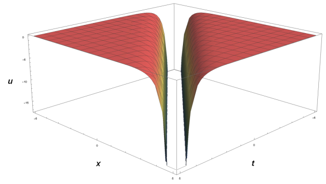
In this article, the generalized $ \left(N+1\right) $-dimensional nonlinear Boussinesq equation is analyzed via Lie symmetry method. Lie point symmetries of the considered equation and accompanying invariant groups are computed. After transforming the equation into a nonlinear ordinary differential equation (ODE), analytical solutions of various types are obtained using the $ \left(G^\prime/G, 1/G\right) $ expansion method. The concept of nonlinear self-adjointness is used in order to determine nonlocal conservation laws of the equation in lower dimensions. By selecting the appropriate parameter values, the study provides a graph of the solutions to the equation under study.
- generalized Boussinesq equation,
- Lie symmetry analysis,
- nonlinear self-adjointness,
- $ \left(G^\prime/G, 1/G\right) $ expansion method,
- conservation laws
Citation: Amjad Hussain, Muhammad Khubaib Zia, Kottakkaran Sooppy Nisar, Velusamy Vijayakumar, Ilyas Khan. Lie analysis, conserved vectors, nonlinear self-adjoint classification and exact solutions of generalized $ \left(N+1\right) $-dimensional nonlinear Boussinesq equation[J]. AIMS Mathematics, 2022, 7(7): 13139-13168. doi: 10.3934/math.2022725

Related Papers:

Abstract

In this article, the generalized $ \left(N+1\right) $-dimensional nonlinear Boussinesq equation is analyzed via Lie symmetry method. Lie point symmetries of the considered equation and accompanying invariant groups are computed. After transforming the equation into a nonlinear ordinary differential equation (ODE), analytical solutions of various types are obtained using the $ \left(G^\prime/G, 1/G\right) $ expansion method. The concept of nonlinear self-adjointness is used in order to determine nonlocal conservation laws of the equation in lower dimensions. By selecting the appropriate parameter values, the study provides a graph of the solutions to the equation under study.

References

[1]	J. Boussinesq, Théorie des ondes et des remous qui se propagent le long d'un canal rectangulaire horizontal, en communiquant au liquide contenu dans ce canal des vitesses sensiblement pareilles de la surface au fond, J. Math. Pure. Appl., 1872, 55–108.
[2]	Y. L. Ma, A. M. Wazwaz, B. Q. Li, Novel bifurcation solitons for an extended Kadomtsev-Petviashvili equation in fluids, Phys. Lett. A, 413 (2021), 127585. https://doi.org/10.1016/j.physleta.2021.127585 doi: 10.1016/j.physleta.2021.127585
[3]	B. Q. Li, New breather and multiple-wave soliton dynamics for generalized Vakhnenko-Parkes equation with variable coefficients, J. Comput. Nonlinear Dyn., 16 (2021), 091006. https://doi.org/10.1115/1.4051624 doi: 10.1115/1.4051624
[4]	Y. L. Ma, A. M. Wazwaz, B. Q. Li, A new (3+1)-dimensional Kadomtsev-Petviashvili equation and its integrability, multiple-solitons, breathers and lump waves, Math. Comput. Simul., 187 (2021), 505–519. https://doi.org/10.1016/j.matcom.2021.03.012 doi: 10.1016/j.matcom.2021.03.012
[5]	B. Q. Li, Loop-like kink breather and its transition phenomena for the Vakhnenko equation arising from high-frequency wave propagation in electromagnetic physics, Appl. Math. Lett., 112 (2021), 106822. https://doi.org/10.1016/j.aml.2020.106822 doi: 10.1016/j.aml.2020.106822
[6]	Y. L. Ma, A. M. Wazwaz, B. Q. Li, New extended Kadomtsev-Petviashvili equation: Multiple soliton solutions, breather, lump and interaction solutions, Nonlinear Dynam., 104 (2021), 1581–1594. https://doi.org/10.1007/s11071-021-06357-8 doi: 10.1007/s11071-021-06357-8
[7]	M. N. Alam, M. A. Akbar, S. T. Mohyud-Din, A novel $G^{\prime}/G$-expansion method and its application to the Boussinesq equation, Chinese Phys. B, 23 (2013).
[8]	X. Lü, J. P. Wang, F. H. Lin, X. W. Zhou, Lump dynamics of a generalized two-dimensional Boussinesq equation in shallow water, Nonlinear Dynam., 91 (2018), 1249–1259. https://doi.org/10.1007/s11071-017-3942-y doi: 10.1007/s11071-017-3942-y
[9]	A. M. Jawad, M. Petković, P. Laketa, A. Biswas, Dynamics of shallow water waves with Boussinesq equation, Sci. Iran., 20 (2013), 179–184. https://doi.org/10.1016/j.scient.2012.12.011 doi: 10.1016/j.scient.2012.12.011
[10]	S. Rashid, K. T. Kubra, H. Jafari, S. U. Lehre, A semi-analytical approach for fractional order Boussinesq equation in a gradient unconfined aquifers, Math. Method. Appl. Sci., 45 (2021), 1033–1062. https://doi.org/10.1002/mma.7833 doi: 10.1002/mma.7833
[11]	M. A. Akbar, N. H. M. Ali, T. Tanjim, Adequate soliton solutions to the perturbed Boussinesq equation and the KdV-Caudrey-Dodd-Gibbon equation, J. King Saud Univ. Sci., 32 (2020), 2777–2785. https://doi.org/10.1016/j.jksus.2020.06.014 doi: 10.1016/j.jksus.2020.06.014
[12]	Y. L. Ma, B. Q. Li, Analytic rogue wave solutions for a generalized fourth-order Boussinesq equation in fluid mechanics, Math. Method. Appl. Sci., 42 (2019), 39–48. https://doi.org/10.1002/mma.5320 doi: 10.1002/mma.5320
[13]	Y. L. Ma, N-solitons, breathers and rogue waves for a generalized Boussinesq equation, Int. J. Comput. Math., 97 (2020), 648–1661. https://doi.org/10.1080/00207160.2019.1639678 doi: 10.1080/00207160.2019.1639678
[14]	Y. L. Ma, B. Q. Li, Bifurcation solitons and breathers for the nonlocal Boussinesq equations, Appl. Math. Lett., 124 (2020), 107677. https://doi.org/10.1016/j.aml.2021.107677 doi: 10.1016/j.aml.2021.107677
[15]	G. Fal'kovich, M. Spector, S. Turitsyn, Destruction of stationary solutions and collapse in the nonlinear string equation, Phys. Lett. A, 99 (1983), 271–274. https://doi.org/10.1016/0375-9601(83)90882-4 doi: 10.1016/0375-9601(83)90882-4
[16]	G. Morosanu, Nonlinear evolution equations and applications, Springer Science & Business Media, 26 (1988).
[17]	Q. Liu, R. Zhang, L. Yang, J. Song, A new model equation for nonlinear Rossby waves and some of its solutions, Phys. Lett. A, 383 (2019), 514–525. https://doi.org/10.1016/j.physleta.2018.10.052 doi: 10.1016/j.physleta.2018.10.052
[18]	J. Zhang, R. Zhang, L. Yang, Q. Liu, L. Chen, Coherent structures of nonlinear barotropic-baroclinic interaction in unequal depth two-layer model, Appl. Math. Comput., 408 (2021), 126347. https://doi.org/10.1016/j.amc.2021.126347 doi: 10.1016/j.amc.2021.126347
[19]	X. Zhang, H. Zhang, Y. Yang, J. Song, Effect of quadric shear basic zonal flows and topography on baroclinic instability, Tellus A, 72 (2020), 1–9. https://doi.org/10.1080/16000870.2020.1843330 doi: 10.1080/16000870.2020.1843330
[20]	Y. Yang, J. Song, On the generalized eigenvalue problem of Rossby waves vertical velocity under the condition of zonal mean flow and topography, Appl. Math. Lett., 121 (2021), 107485. https://doi.org/10.1016/j.aml.2021.107485 doi: 10.1016/j.aml.2021.107485
[21]	X. L. Gai, Y. T. Gao, X. Yu, Z. Y. Sun, Soliton interactions for the generalized (3+1)-dimensional Boussinesq equation, Int. J. Mod. Phys. B, 26 (2012), 125006. https://doi.org/10.1142/S0217979212500622 doi: 10.1142/S0217979212500622
[22]	Z. Yan, Similarity transformations and exact solutions for a family of higher-dimensional generalized Boussinesq equations, Phys. Lett. A, 361 (2007), 223–230. https://doi.org/10.1016/j.physleta.2006.07.047 doi: 10.1016/j.physleta.2006.07.047
[23]	P. A. Clarkson, M. D. Kruskal, New similarity reductions of the Boussinesq equation, J. Math. Phys., 30 (1989), 2201–2213. https://doi.org/10.1063/1.528613 doi: 10.1063/1.528613
[24]	M. El-Sabbagh, A. Ali, New exact solutions for (3+1)-dimensional Kadomtsev-Petviashvili equation and generalized (2+1)-dimensional Boussinesq equation, Int. J. Nonlinear Sci. Numer. Simul., 6 (2005), 151–162. https://doi.org/10.1515/IJNSNS.2005.6.2.151 doi: 10.1515/IJNSNS.2005.6.2.151
[25]	X. W. Yan, Generalized (3+1)-dimensional Boussinesq equation: Breathers, rogue waves and their dynamics, Mod. Phys. Lett. B, 34 (2020), 2050003. https://doi.org/10.1142/S0217984920500037 doi: 10.1142/S0217984920500037
[26]	W. X. Ma, C. X. Li, J. He, A second Wronskian formulation of the Boussinesq equation, Nonlinear Anal.-Theor., 70 (2009), 4245–4258. https://doi.org/10.1016/j.na.2008.09.010 doi: 10.1016/j.na.2008.09.010
[27]	H. Zhang, B. Tian, H. Q. Zhang, T. Geng, X. H. Meng, W. J. Liu, et al., Periodic wave solutions for (2+1)-dimensional Boussinesq equation and (3+1)-dimensional Kadomtsev-Petviashvili equation, Commun. Theor. Phys., 50 (2008), 1169.
[28]	W. Y. Sun, Y. Y. Sun, The degenerate breather solutions for the Boussinesq equation, Appl. Math. Lett., 128 (2022), 107884. https://doi.org/10.1016/j.aml.2021.107884 doi: 10.1016/j.aml.2021.107884
[29]	M. Parvizi, A. Khodadadian, M. Eslahchi, Analysis of Ciarlet-Raviart mixed finite element methods for solving damped Boussinesq equation, J. Comput. Appl. Math., 379 (2020), 112818. https://doi.org/10.1016/j.cam.2020.112818 doi: 10.1016/j.cam.2020.112818
[30]	Y. Liu, B. Li, A. M. Wazwaz, Novel high-order breathers and rogue waves in the Boussinesq equation via determinants, Math. Method. Appl. Sci., 43 (2020), 3701–3715. https://doi.org/10.1002/mma.6148 doi: 10.1002/mma.6148
[31]	D. J. Ratliff, Double degeneracy in multiphase modulation and the emergence of the Boussinesq equation, Stud. Appl. Math., 140 (2018), 48–77. https://doi.org/10.1111/sapm.12189 doi: 10.1111/sapm.12189
[32]	M. T. Darvishi, M. Najafi, A. M. Wazwaz, Traveling wave solutions for Boussinesq-like equations with spatial and spatial-temporal dispersion, Rom. Rep. Phys., 70 (2018), 108.
[33]	A. Zafar, H. Rezazadeh, W. Reazzaq, A. Bekir, The simplest equation approach for solving non-linear Tzitzéica type equations in non-linear optics, Mod. Phys. Lett. B, 35 (2021). https://doi.org/10.1142/S0217984921501323
[34]	M. Ekici, M. Mirzazadeh, A. Sonmezoglu, M. Z. Ullah, Q. Zhou, H. Triki, et al., Optical solitons with anti-cubic nonlinearity by extended trial equation method, Optik, 136 (2017), 368–373. https://doi.org/10.1016/j.ijleo.2017.02.004 doi: 10.1016/j.ijleo.2017.02.004
[35]	H. Durur, E. Ilhan, H. Bulut, Novel complex wave solutions of the (2+1)-dimensional hyperbolic nonlinear Schrödinger equation, Fractal Fract., 4 (2020), 41. https://doi.org/10.3390/fractalfract4030041 doi: 10.3390/fractalfract4030041
[36]	A. Hussain, A. Jhangeer, S. Tahir, Y. M. Chu, I. Khan, K. S. Nisar, Dynamical behavior of fractional Chen-Lee-Liu equation in optical fibers with beta derivatives, Results Phys., 18 (2020). https://doi.org/10.1016/j.rinp.2020.103208
[37]	A. Jhangeer, A. Hussain, S. Tahir, S. Sharif, Solitonic, super nonlinear, periodic, quasiperiodic, chaotic waves and conservation laws of modified Zakharov-Kuznetsov equation in transmission line, Commun. Nonlinear Sci. Numer. Simul., 86 (2020). https://doi.org/10.1016/j.cnsns.2020.105254
[38]	A. Hussain, M. Junaid-U-Rehman, F. Jabeen, I. Khan, Optical solitons of NLS-type differential equations by extended direct algebraic method, Int. J. Geom. Methods Mod. Phys., 19 (2022). https://doi.org/10.1142/S021988782250075X
[39]	M. A. H. Khaled, M. A. Shukri, Y. A. U. Hager, Dust acoustic multi-soliton collisions in a dusty plasma using Hirota bilinear method, J. Amr. Uni., 1 (2021), 129.
[40]	A. S. Bezgabadi, M. Bolorizadeh, Analytic combined bright-dark, bright and dark solitons solutions of generalized nonlinear Schrödinger equation using extended Sinh-Gordon equation expansion method, Results Phys., 30 (2021), 104852. https://doi.org/10.1016/j.rinp.2021.104852 doi: 10.1016/j.rinp.2021.104852
[41]	Y. Bi, Z. Zhang, Q. Liu, T. Liu, Research on nonlinear waves of blood flow in arterial vessels, Commun. Nonlinear Sci. Numer. Simul., 102 (2021). https://doi.org/10.1016/j.cnsns.2021.105918
[42]	B. Elma, E. Mısırlı, Applications of the extended exp (- $\phi$ ($\xi$))-expansion method to some non-linear fractional evolution equations, In 9th (Online) International Conference on Applied Analysis and Mathematical Modeling (ICAAMM21), Istanbul-Turkey, 2021, 17.
[43]	Y. L. Zhao, Y. P. Liu, Z. B. Li, A connection between the ($G^{\prime}/G$)-expansion method and the truncated Painlevé expansion method and its application to the mKdV equation, Chinese Phys. B, 19 (2010).
[44]	J. Li, Y. Qiu, D. Lu, R. A. Attia, M. Khater, Study on the solitary wave solutions of the ionic currents on microtubules equation by using the modified Khater method, Therm. Sci., 23 (2019), 2053–2062. https://doi.org/10.2298/TSCI190722370L doi: 10.2298/TSCI190722370L
[45]	H. M. Ahmed, W. B. Rabie, M. A. Ragusa, Optical solitons and other solutions to Kaup-Newell equation with Jacobi elliptic function expansion method, Anal. Math. Phys., 11 (2021), 1–16. https://doi.org/10.1007/s13324-020-00464-2 doi: 10.1007/s13324-020-00464-2
[46]	P. E. Hydon, P. E. Hydon, Symmetry methods for differential equations: A beginner's guide, Cambridge University Press, 2000.
[47]	D. J. Arrigo, Symmetry analysis of differential equations: An introduction, John Wiley & Sons, 2015.
[48]	A. Hussain, A. Jhangeer, N. Abbas, I. Khan, K. S. Nisar, Solitary wave patterns and conservation laws of fourth-order nonlinear symmetric regularized long-wave equation arising in plasma, Ain Shams Eng. J., 12 (2021), 3919–3930. https://doi.org/10.1016/j.asej.2020.11.029 doi: 10.1016/j.asej.2020.11.029
[49]	S. Kumar, M. Niwas, A. M. Wazwaz, Lie symmetry analysis, exact analytical solutions and dynamics of solitons for (2+1)-dimensional NNV equations, Phys. Scripta, 95 (2020).
[50]	A. Hussain, A. Jhangeer, N. Abbas, Symmetries, conservation laws and dust acoustic solitons of two-temperature ion in inhomogeneous plasma, Int. J. Geom. Methods Mod. Phys., 18 (2021). https://doi.org/10.1142/S0219887821500717
[51]	M. R. Ali, W. X. Ma, R. Sadat, Lie symmetry analysis and invariant solutions for (2+1)-dimensional Bogoyavlensky-Konopelchenko equation with variable-coefficient in wave propagation, J. Ocean Eng. Sci., 2021. https://doi.org/10.1016/j.joes.2021.08.006
[52]	A. Hussain, S. Bano, I. Khan, D. Baleanu, K. Sooppy Nisar, Lie symmetry analysis, explicit solutions and conservation laws of a spatially two-dimensional Burgers-Huxley equation, Symmetry, 12 (2020), 170. https://doi.org/10.3390/sym12010170 doi: 10.3390/sym12010170
[53]	K. Sethukumarasamy, P. Vijayaraju, P. Prakash, On Lie symmetry analysis of certain coupled fractional ordinary differential equations, J. Nonlinear Math. Phys., 28 (2021), 219–241. https://doi.org/10.2991/jnmp.k.210315.001 doi: 10.2991/jnmp.k.210315.001
[54]	A. Jhangeer, A. Hussain, M. Junaid-U-Rehman, I. Khan, D. Baleanu, K. S. Nisar, Lie analysis, conservation laws and travelling wave structures of nonlinear Bogoyavlenskii-Kadomtsev-Petviashvili equation, Results Phys., 19 (2020). https://doi.org/10.1016/j.rinp.2020.103492
[55]	D. Yu, Z. G. Zhang, H. H. Dong, H. W. Yang, Bäcklund transformation, infinite number of conservation laws and fission properties of an integro-differential model for ocean internal solitary waves, Commun. Theor. Phys., 73 (2021). https://doi.org/10.1088/1572-9494/abda1e
[56]	R. Naz, F. M. Mahomed, D. P. Mason, Comparison of different approaches to conservation laws for some partial differential equations in fluid mechanics, Appl. Math. Comput., 205 (2008), 212–230. https://doi.org/10.1016/j.amc.2008.06.042 doi: 10.1016/j.amc.2008.06.042
[57]	M. B. Riaz, D. Baleanu, A. Jhangeer, N. Abbas, Nonlinear self-adjointness, conserved vectors, and traveling wave structures for the kinetics of phase separation dependent on ternary alloys in iron (Fe-Cr-Y (Y = Mo, Cu)), Results Phys., 25 (2021), 104151. https://doi.org/10.1016/j.rinp.2021.104151 doi: 10.1016/j.rinp.2021.104151
[58]	M. Inc, A. I. Aliyu, A. Yusuf, D. Baleanu, Combined optical solitary waves and conservation laws for nonlinear Chen-Lee-Liu equation in optical fibers, Optik, 158 (2018), 297–304. https://doi.org/10.1016/j.ijleo.2017.12.075 doi: 10.1016/j.ijleo.2017.12.075
[59]	C. M. Khalique, O. D. Adeyemo, A study of (3+1)-dimensional generalized Korteweg-de Vries-Zakharov-Kuznetsov equation via Lie symmetry approach, Results Phys., 18 (2020). https://doi.org/10.1016/j.rinp.2020.103197
[60]	C. Fu, C. N. Lu, H. W. Yang, Timespace fractional (2+1)-dimensional nonlinear Schrödinger equation for envelope gravity waves in baroclinic atmosphere and conservation laws as well as exact solutions, Adv. Diff. Equ., 2018 (2018), 1–20. https://doi.org/10.1186/s13662-018-1512-3 doi: 10.1186/s13662-018-1512-3
[61]	N. H. Ibragimov, Nonlinear self-adjointness and conservation laws, J. Phys. A, 44 (2021). https://doi.org/10.1088/1751-8113/44/43/432002
[62]	M. Gandarias, Weak self-adjoint differential equations, J. Phys. A, 44 (2011). https://doi.org/10.1088/1751-8113/44/26/262001
[63]	S. F. Tian, Lie symmetry analysis, conservation laws and solitary wave solutions to a fourth-order nonlinear generalized Boussinesq water wave equation, Appl. Math. Lett., 100 (2020). https://doi.org/10.1016/j.aml.2019.106056
[64]	M. J. Xu, S. F. Tian, J. M. Tu, T. T. Zhang, Bäcklund transformation, infinite conservation laws and periodic wave solutions to a generalized (2+1)-dimensional Boussinesq equation, Nonlinear Anal.-Real, 31 (2016), 388–408. https://doi.org/10.1016/j.nonrwa.2016.01.019 doi: 10.1016/j.nonrwa.2016.01.019

Reader Comments

Your name:*

Email:*
© 2022 the Author(s), licensee AIMS Press. This is an open access article distributed under the terms of the Creative Commons Attribution License (http://creativecommons.org/licenses/by/4.0)