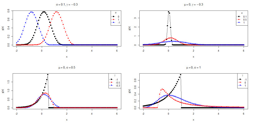
Analyzing the statistical behavior of the assets' returns has shown to be an interesting approach to perform asset selection. In this work, we explore a stress-strength reliability approach to perform asset selection based on probabilities of the type $ P(X < Y) $ when both $ X $ and $ Y $ follow a generalized extreme value (GEV) distribution with three parameters. At first, we derive new analytical and closed form relations in terms of the extreme value $ \mathbb{H} $-function, which have been obtained under fewer parameter restrictions compared to similar results in the literature. To show the performance of our results, we include a Monte-Carlo simulation study and we investigate the application of the reliability measure $ P(X < Y) $ in selecting financial assets with returns characterized by the distributions $ X $ and $ Y $. Therefore, rather than the conventional approach of comparing the expected values of $ X $ and $ Y $ based on modern portfolio theory, we delve into the metric $ P(X < Y) $ as an alternative parameter for assessing better returns.
Citation: Felipe S. Quintino, Melquisadec Oliveira, Pushpa N. Rathie, Luan C. S. M. Ozelim, Tiago A. da Fonseca. Asset selection based on estimating stress-strength probabilities: The case of returns following three-parameter generalized extreme value distributions[J]. AIMS Mathematics, 2024, 9(1): 2345-2368. doi: 10.3934/math.2024116
Analyzing the statistical behavior of the assets' returns has shown to be an interesting approach to perform asset selection. In this work, we explore a stress-strength reliability approach to perform asset selection based on probabilities of the type $ P(X < Y) $ when both $ X $ and $ Y $ follow a generalized extreme value (GEV) distribution with three parameters. At first, we derive new analytical and closed form relations in terms of the extreme value $ \mathbb{H} $-function, which have been obtained under fewer parameter restrictions compared to similar results in the literature. To show the performance of our results, we include a Monte-Carlo simulation study and we investigate the application of the reliability measure $ P(X < Y) $ in selecting financial assets with returns characterized by the distributions $ X $ and $ Y $. Therefore, rather than the conventional approach of comparing the expected values of $ X $ and $ Y $ based on modern portfolio theory, we delve into the metric $ P(X < Y) $ as an alternative parameter for assessing better returns.

| [1] | H. Markowitz, Portfolio selection: Efficient diversification of investments, John Wiley & Sons, 1959. |
| [2] |
M. Rubinstein, Markowitz's "portfolio selection": A fifty-year retrospective, J. Financ., 57 (2002), 1041–1045. https://doi.org/10.1111/1540-6261.00453 doi: 10.1111/1540-6261.00453

|
| [3] | H. Markowitz, Portfolio selection, J. Financ., 7 (1952), 77–91. https://doi.org/10.1111/j.1540-6261.1952.tb01525.x |
| [4] |
W. Sharpe, A simplified model for portfolio analysis, Manag. Sci., 9 (1963), 277–293. https://doi.org/10.1287/mnsc.9.2.277 doi: 10.1287/mnsc.9.2.277
|
| [5] | L. Bachelier, Theorie de la speculation, Doctor Thesis, The Random Character Of Stock Market Prices, Annales Scientifiques Ecole Normale Sperieure III-17, 1900. https://doi.org/10.24033/asens.476 |
| [6] | P. Embrechts, C. Klüppelberg, T. Mikosch, Modelling extremal events: For insurance and finance, Springer Science & Business Media, 2013. |
| [7] | N. N. Taleb, Statistical consequences of fat tails, technical incerto, STEM Academic Press, 2020. |
| [8] | B. Mandelbrot, The variation of some other speculative prices, J. Bus., 40 (1967), 393–413. Available from: http://www.jstor.org/stable/2351623. |
| [9] | A. Jenkinson, The frequency distribution of the annual maximum (or minimum) values of meteorological elements, Q. J. Roy. Meteor. Soc., 81 (1955), 158–171. |
| [10] |
P. Cirillo, N. N. Taleb, Expected shortfall estimation for apparently infinite-mean models of operational risk, Quant. Financ., 16 (2016), 1485–1494. https://doi.org/10.1080/14697688.2016.1162908 doi: 10.1080/14697688.2016.1162908
|
| [11] |
G. D. Gettinby, C. D. Sinclair, D. M. Power, R. A. Brown, An analysis of the distribution of extreme share returns in the UK from 1975 to 2000, J. Bus. Finan. Account., 31 (2004), 607–646. https://doi.org/10.1111/j.0306-686X.2004.00551.x doi: 10.1111/j.0306-686X.2004.00551.x
|
| [12] |
S. I. Hussain, S. Li, Modeling the distribution of extreme returns in the Chinese stock market, J. Int. Financ. Mark. I., 34 (2015), 263–276. https://doi.org/10.1016/j.intfin.2014.11.007 doi: 10.1016/j.intfin.2014.11.007
|
| [13] |
R. Gencay, F. Selçuk, Extreme value theory and Value-at-Risk: Relative performance in emerging markets, Int. J. Forecasting, 20 (2004), 287–303. https://doi.org/10.1016/j.ijforecast.2003.09.005 doi: 10.1016/j.ijforecast.2003.09.005
|
| [14] | J. Galambos, The asymptotic theory of extreme order statistics, R. E. Krieger Publishing Company, 1987. |
| [15] | L. Haan, A. Ferreira, Extreme value theory: An introduction, Springer, 2006. https://doi.org/10.1007/0-387-34471-3 |
| [16] | S. Resnick, Extreme values, regular variation, and point processes, Springer Science & Business Media, 2008. |
| [17] |
R. Fisher, L. Tippett, Limiting forms of the frequency distribution of the largest or smallest member of a sample, Math. Proc. Cambridge, 24 (1928), 180–190. https://doi.org/10.1017/S0305004100015681 doi: 10.1017/S0305004100015681
|
| [18] |
A. Goncu, A. K. Akgul., O. Imamoglu, M. Tiryakioglu, An analysis of the extreme returns distribution: The case of the Istanbul Stock Exchange, Appl. Financ. Econ., 22 (2012), 723–732. https://doi.org/10.1080/09603107.2011.624081 doi: 10.1080/09603107.2011.624081
|
| [19] | S. Kotz, Y. Lumelskii, M. Pensky, The stress-strength model and its generalizations: Theory and applications, World Scientific, 2003. https://doi.org/10.1142/9789812564511 |
| [20] |
F. Domma, S. Giordano, A stress-strength model with dependent variables to measure household financial fragility, Stat. Method. Appl., 21 (2012), 375–389. https://doi.org/10.1007/s10260-012-0192-5 doi: 10.1007/s10260-012-0192-5
|
| [21] | L. C. S. M. Ozelim, C. E. G. Otiniano, P. N. Rathie, On the linear combination of n logistic random variables and reliability analysis, South East Asian J. Math. Math. Sci., 12 (2016), 19–34. |
| [22] |
P. N. Rathie, L. C. S. M. Ozelim, Exact and approximate expressions for the reliability of stable Lévy random variables with applications to stock market modelling, J. Comput. Appl. Math., 321 (2017), 314–322. https://doi.org/10.1016/j.cam.2017.02.043 doi: 10.1016/j.cam.2017.02.043
|
| [23] |
L. C. S. M. Ozelim, P. N. Rathie, Linear combination and reliability of generalized logistic random variables, Eur. J. Pure Appl. Math., 12 (2019), 722–733. https://doi.org/10.29020/nybg.ejpam.v12i3.3444 doi: 10.29020/nybg.ejpam.v12i3.3444
|
| [24] |
P. N. Rathie, L. C. S. M. Ozelim, B. B. Andrade, Portfolio management of copula-dependent assets based on $P(Y < X)$ reliability models: Revisiting Frank copula and Dagum distributions, Stats, 4 (2021), 1027–1050. https://doi.org/10.3390/stats4040059 doi: 10.3390/stats4040059
|
| [25] |
S. Nadarajah, Reliability for extreme value distributions, Math. Comput. Model., 37 (2003), 915–922. https://doi.org/10.1016/S0895-7177(03)00107-9 doi: 10.1016/S0895-7177(03)00107-9
|
| [26] |
K. Krishnamoorthy, Y. Lin, Confidence limits for stress-strength reliability involving Weibull models, J. Stat. Plan. Infer., 140 (2010), 1754–1764. https://doi.org/10.1016/j.jspi.2009.12.028 doi: 10.1016/j.jspi.2009.12.028
|
| [27] |
D. Kundu, M. Raqab, Estimation of $R = P (Y < X)$ for three-parameter Weibull distribution, Stat. Probabil. Lett., 79 (2009), 1839–1846. https://doi.org/10.1016/j.spl.2009.05.026 doi: 10.1016/j.spl.2009.05.026
|
| [28] |
R. Nojosa, P. N. Rathie, Stress-strength reliability models involving generalized gamma and Weibull distributions, Int. J. Qual. Reliab. Ma., 37 (2020), 538–551. https://doi.org/10.1108/IJQRM-06-2019-0190 doi: 10.1108/IJQRM-06-2019-0190
|
| [29] |
K. Abbas, Y. Tang, Objective Bayesian analysis of the Frechet stress-strength model, Stat. Probabil. Lett., 84 (2014), 169–175. https://doi.org/10.1016/j.spl.2013.09.014 doi: 10.1016/j.spl.2013.09.014
|
| [30] |
X. Jia, S. Nadarajah, B. Guo, Bayes estimation of $P(Y < X)$ for the Weibull distribution with arbitrary parameters, Appl. Math. Model., 47 (2017), 249–259. https://doi.org/10.1016/j.apm.2017.03.020 doi: 10.1016/j.apm.2017.03.020
|
| [31] | P. N. Rathie, L. C. S. M. Ozelim, F. Quintino, T. Fonseca, On the extreme value H-function, Stats, 6 (2023), 802–811. Available from: https://www.mdpi.com/2571-905X/6/3/51. |
| [32] | A. Mathai, R. Saxena, H. Haubold, The H-function: Theory and applications, Springer Science & Business Media, 2009. |
| [33] | P. N. Rathie, S. Freitas, R. Nojosa, A. Mendes, T. Silva, Stress-strength reliability models involving H-function distributions, J. Ramanu. Soc. Math. Math. Sci., 9 (2022), 217–234. |
| [34] | R. C. Team, R: A language and environment for statistical computing, R Found. Stat. Comput., 2022. Available from: https://www.R-project.org/. |


Figures(6) / Tables(15)

Felipe S. Quintino, Melquisadec Oliveira, Pushpa N. Rathie, Luan C. S. M. Ozelim, Tiago A. da Fonseca. Asset selection based on estimating stress-strength probabilities: The case of returns following three-parameter generalized extreme value distributions[J]. AIMS Mathematics, 2024, 9(1): 2345-2368. doi: 10.3934/math.2024116


 DownLoad: