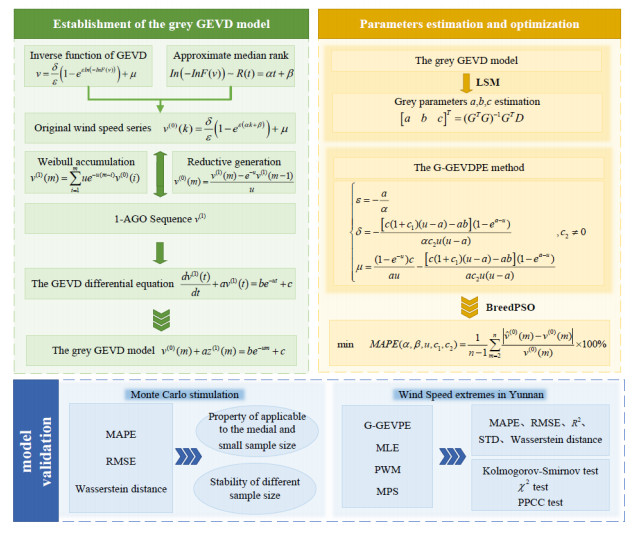
Accurate parameter estimation of extreme wind speed distribution is of great importance for the safe utilization and assessment of wind resources. This paper emphatically establishes a novel grey generalized extreme value method for parameter estimation of annual wind speed extremum distribution (AWSED). Considering the uncertainty and frequency characteristics of the parent wind speed, the generalized extreme value distribution (GEVD) is selected as the probability distribution, and the Weibull distribution is utilized as the first-order accumulation generating operator. Then, the GEVD differential equation is derived, and it is transformed into the grey GEVD model using the differential information principle. The least squares method is used to estimate the grey GEVD model parameters, and then a novel estimation method is proposed through grey parameters. A hybrid particle swarm optimization algorithm is used to optimize distribution parameters. The novel method is stable under different sample sizes according to Monte Carlo comparison simulation results, and the suitability for the novel method is confirmed by instance analysis in Wujiaba, Yunnan Province. The new method performs with high accuracy in various indicators, the hypothesis test results are above 95%, and the statistical errors such as MAPE and Wasserstein distance yield the lowest, which are 3.33% and 0.2556, respectively.
Citation: Yichen Lv, Xinping Xiao. Grey parameter estimation method for extreme value distribution of short-term wind speed data[J]. AIMS Mathematics, 2024, 9(3): 6238-6265. doi: 10.3934/math.2024304
Accurate parameter estimation of extreme wind speed distribution is of great importance for the safe utilization and assessment of wind resources. This paper emphatically establishes a novel grey generalized extreme value method for parameter estimation of annual wind speed extremum distribution (AWSED). Considering the uncertainty and frequency characteristics of the parent wind speed, the generalized extreme value distribution (GEVD) is selected as the probability distribution, and the Weibull distribution is utilized as the first-order accumulation generating operator. Then, the GEVD differential equation is derived, and it is transformed into the grey GEVD model using the differential information principle. The least squares method is used to estimate the grey GEVD model parameters, and then a novel estimation method is proposed through grey parameters. A hybrid particle swarm optimization algorithm is used to optimize distribution parameters. The novel method is stable under different sample sizes according to Monte Carlo comparison simulation results, and the suitability for the novel method is confirmed by instance analysis in Wujiaba, Yunnan Province. The new method performs with high accuracy in various indicators, the hypothesis test results are above 95%, and the statistical errors such as MAPE and Wasserstein distance yield the lowest, which are 3.33% and 0.2556, respectively.

| [1] |
B. Kresning, M. Hashemi, A. Shirvani, J. Hashemi, Uncertainty of extreme wind and wave loads for marine renewable energy farms in hurricane-prone regions, Renew. Energ., 220 (2024), 119570. https://doi.org/10.1016/j.renene.2023.119570 doi: 10.1016/j.renene.2023.119570

|
| [2] |
L. Da, Q. Yang, M. Liu, L. Zhao, T. Wu, B. Chen, Estimation of extreme wind speed based on upcrossing rate of mean wind speeds with Weibull distribution, J. Wind Eng. Ind. Aerod., 240 (2023), 105495. https://doi.org/10.1016/j.jweia.2023.105495 doi: 10.1016/j.jweia.2023.105495
|
| [3] |
Y. Charabi, S. Abdul-Wahab, A. M. Al-Mahruqi, S. Osman, I. Osman, The potential estimation and cost analysis of wind energy production in Oman, Environ. Dev. Sustain., 24 (2022), 5917–5937. https://doi.org/10.1007/s10668-021-01692-7 doi: 10.1007/s10668-021-01692-7
|
| [4] | International Standard IEC61400-1, International Electrotechnical Commission, 2005. Available from: https://webstore.iec.ch/preview/info_iec61400-1%7Bed3.0%7Den.pdf. |
| [5] |
M. Abdelwahab, T. Ghazal, K. Nadeem, A. Haitham, E. Ahmed, Performance-based wind design for tall buildings: Review and comparative study, J. Build. Eng., 68 (2023), 106103. https://doi.org/10.1016/j.jobe.2023.106103 doi: 10.1016/j.jobe.2023.106103
|
| [6] |
H. C. S. Thom, Distributions of extreme winds in the United States, Journal of the Structural Division, 86 (1960), 11–24. https://doi.org/10.1061/TACEAT.0008243 doi: 10.1061/TACEAT.0008243
|
| [7] |
E. Simiu, M. ASCE, J. Biétry, J. J. Filliben, Sampling errors in estimation of extreme winds, Journal of the Structural Division, 104 (1978), 491–501. https://doi.org/10.1061/JSDEAG.0004882 doi: 10.1061/JSDEAG.0004882
|
| [8] | National Wind Energy Resources Evaluation Technical Regulations, 2004. Available from: http://www.nea.gov.cn/201201/04/c_131260326.html. |
| [9] |
E. Simiu, M. ASCE, M. J. Changery, J. J. Filliben, Extreme wind speeds at 129 airport stations, Journal of the Structural Division, 106 (1980), 809–817. https://doi.org/10.1061/JSDEAG.0005399 doi: 10.1061/JSDEAG.0005399
|
| [10] |
E. Simiu, M. ASCE, J. J. Filliben, Probability distributions of extreme wind speeds, Journal of the Structural Division, 102 (1976), 1861–1877. https://doi.org/10.1061/JSDEAG.0004434 doi: 10.1061/JSDEAG.0004434
|
| [11] | A. P. Lu, L. Zhao, Z. W. Guo, Y. J. Ge, A comparative study of extreme value distribution and parameter estimation based on the Monte Carlo method, Journal of Harbin Institute of Technology, 45 (2013), 88–95. |
| [12] |
A. F. Jenkinson, The frequency distribution of the annual maximum (or minimum) values of meteorological elements, Q. J. Roy. Meteor. Soc., 81 (1955), 158–171. https://doi.org/10.1002/qj.49708134804 doi: 10.1002/qj.49708134804
|
| [13] |
R. W. Katz, M. B. Parlange, P. Naveau, Statistics of extremes in hydrology, Adv. Water Resour., 25 (2002), 1287–1304. https://doi.org/10.1016/S0309-1708(02)00056-8 doi: 10.1016/S0309-1708(02)00056-8
|
| [14] |
H. Madsen, P. F. Rasmussen, D. Rosbjerg, Comparison of annual maximum series and partial duration series methods for modeling extreme hydrologic events: 1. At‐site modeling, Water Resour. Res., 33 (1997), 747–757. https://doi.org/10.1029/96WR03848 doi: 10.1029/96WR03848
|
| [15] |
E. Castillo, A. S. Hadi, Parameter and quantile estimation for the generalized extreme-value distribution, Environmetrics, 5 (1994), 417–432. https://doi.org/10.1002/env.3170050405 doi: 10.1002/env.3170050405
|
| [16] |
S. D. Nerantzaki, S. M. Papalexiou, Assessing extremes in hydroclimatology: A review on probabilistic methods, J. Hydrol., 605 (2022), 127302. https://doi.org/10.1016/j.jhydrol.2021.127302 doi: 10.1016/j.jhydrol.2021.127302
|
| [17] | N. M. Xie, R. Z. Wang, A historic review of grey forecasting models, The Journal of Grey System, 29 (2017), 1–29. |
| [18] |
W. Lei, S. Mao, Y. Zhang, Estimating China's CO2 emissions under the influence of COVID-19 epidemic using a novel fractional multivariate nonlinear grey model, Environ. Dev. Sustain., 2023 (2023), 1–32. https://doi.org/10.1007/s10668-023-03325-7 doi: 10.1007/s10668-023-03325-7
|
| [19] |
Q. Z. Xiao, M. Y. Gao, L. Chen, J. C. Jiang, Dynamic multi-attribute evaluation of digital economy development in China: A perspective from interaction effect, Tech. Econ. Dev. Eco., 29 (2023), 1728–1752. https://doi.org/10.3846/tede.2023.20258 doi: 10.3846/tede.2023.20258
|
| [20] |
S. W. Wang, X. P. Xiao, Q. Ding, A novel fractional system grey prediction model with dynamic delay effect for evaluating the state of health of lithium battery, Energy, 290 (2024), 130057. https://doi.org/10.1016/j.energy.2023.130057 doi: 10.1016/j.energy.2023.130057
|
| [21] |
P. Prescott, A. T. Walden, Maximum likelihood estimation of the parameters of the generalized extreme-value distribution, Biometrika, 67 (1980), 723–724. https://doi.org/10.1093/biomet/67.3.723 doi: 10.1093/biomet/67.3.723
|
| [22] |
E. S. Martins, J. R. Stedinger, Generalized maximum-likelihood generalized extreme-value quantile estimators for hydrologic data, Water Resour. Res., 36 (2000), 737–744. https://doi.org/10.1029/1999WR900330 doi: 10.1029/1999WR900330
|
| [23] |
N. Papukdee, J. S. Park, P. Busababodhin, Penalized likelihood approach for the four-parameter kappa distribution, J. Appl. Stat., 49 (2022), 1559–1573. https://doi.org/10.1080/02664763.2021.1871592 doi: 10.1080/02664763.2021.1871592
|
| [24] | A. J. Cannon, An intercomparison of regional and at-site rainfall extreme value analyses in southern British Columbia, Canada, Can. J. Civil Eng., 42 (2015), 107–119. https://doi.org/10.1139/cjce-2014-0361 |
| [25] |
X. Yang, L. Xie, B. Zhao, X. Kong, N. Wu, An iterative method for parameter estimation of the three-parameter Weibull distribution based on a small sample size with a fixed shape parameter, Int. J. Struct. Stab. Dy., 22 (2022), 2250125. https://doi.org/10.1142/S0219455422501255 doi: 10.1142/S0219455422501255
|
| [26] |
C. T. Lin, Y. Liu, Y. W. Li, Z. W. Chen, H. M. Okasha, Further properties and estimations of exponentiated generalized linear exponential distribution, Mathematics, 9 (2021), 3328. https://doi.org/10.3390/math9243328 doi: 10.3390/math9243328
|
| [27] |
G. P. Sillitto, Interrelations between certain linear systematic statistics of samples from any continuous population, Biometrika, 38 (1951), 377–382. https://doi.org/10.2307/2332583 doi: 10.2307/2332583
|
| [28] |
J. M. Landwehr, N. C. Matalas, J. R. Wallis, Probability weighted moments compared with some traditional techniques in estimating Gumbel Parameters and quantiles, Water Resour. Res., 15 (1979), 1055–1064. https://doi.org/10.1029/WR015i005p01055 doi: 10.1029/WR015i005p01055
|
| [29] |
R. Guan, W. Cheng, Y. Rong, X. Zhao, Parameter estimation of Beta-exponential distribution using linear combination of order statistics, Commun. Math. Stat., 2023 (2023), 1–41. https://doi.org/10.1007/s40304-022-00306-6 doi: 10.1007/s40304-022-00306-6
|
| [30] | M. Shakeel, M. A. Haq, I. Hussain, A. M. Abdulhamid, M. Faisal, Comparison of two new robust parameter estimation methods for the power function distribution, PloS one, 11 (2016), e0160692. https://doi.org/10.1371/journal.pone.0160692 |
| [31] | S. Mahdi, F. Ashkar, Exploring generalized probability weighted moments, generalized moments and maximum likelihood estimating methods in two-parameter Weibull model, J. Hydrol., 285 (2004), 62–75. https://doi.org/10.1016/j.jhydrol.2003.08.012 |
| [32] |
R. C. H. Cheng, N. A. K. Amin, Estimating parameters in continuous univariate distributions with a shifted origin, J. R. Stat. Soc. B, 45 (1983), 394–403. https://doi.org/10.1111/j.2517-6161.1983.tb01268.x doi: 10.1111/j.2517-6161.1983.tb01268.x
|
| [33] | A. M. El Gazar, M. ElGarhy, B. S. El-Desouky, Classical and Bayesian estimation for the truncated inverse power Ailamujia distribution with applications, AIP Adv., 13 (2023), 125122. https://doi.org/10.1063/5.0174794 |
| [34] | Y. M. Kantar, B. Şenoğlu, A comparative study for the location and scale parameters of the Weibull distribution with given shape parameter, Comput. Geosci., 34 (2008), 1900–1909. https://doi.org/10.1016/j.cageo.2008.04.004 |
| [35] | A. Yalçınkaya, U. Yolcu, B. Şenoǧlu, Maximum likelihood and maximum product of spacings estimations for the parameters of skew-normal distribution under doubly type Ⅱ censoring using genetic algorithm, Expert Syst. Appl., 168 (2021), 114407. https://doi.org/10.1016/j.eswa.2020.114407 |
| [36] | M. Z. Anis, I. E. Okorie, M. Ahsanullah, A review of the Rayleigh distribution: properties, estimation & application to COVID-19 data, Bull. Malays. Math. Sci. Soc., 47 (2024), 6. https://doi.org/10.1007/s40840-023-01605-z |
| [37] | R. Y. Zheng, Z. Z. Qin, Grey estimations for the three parameters Weibull distribution, Strength and Environment, 4 (1989), 34–40. |
| [38] |
D. F. Zhao, B. L. Li, S. Lu, J. Wang, Life estimation of chemical machinery based on linear regression and Grey-Weibull model, Chemical Engineering and Machinery, 38 (2011), 517–521. https://doi.org/10.3969/j.issn.0254-6094.2011.05.002 doi: 10.3969/j.issn.0254-6094.2011.05.002
|
| [39] | X. Y. Li, Research on estimation for the three-parameter Weibull distribution, PhD Thesis, Beijing Jiaotong University, 2012. |
| [40] |
X. M. Liu, N. M. Xie, Grey-based approach for estimating Weibull model and its application, Commun. Stat.-Theor. M., 52 (2023), 7601–7617. https://doi.org/10.1080/03610926.2022.2050397 doi: 10.1080/03610926.2022.2050397
|
| [41] |
B. Gao, K. Q. Cao, L. M. Hu, S. G. Li, 3-Parameter Weibull distribution estimation based on GM and SVM, Journal of Mechanical Strength, 40 (2018), 632–638. https://doi.org/10.16579/j.issn.1001.9669.2018.03.021 doi: 10.16579/j.issn.1001.9669.2018.03.021
|
| [42] |
K. Li, P. Xiong, Y. Wu, Y. Dong, Forecasting greenhouse gas emissions with the new information priority generalized accumulative grey model, Sci. Total Environ., 807 (2022), 150859. https://doi.org/10.1016/j.scitotenv.2021.150859 doi: 10.1016/j.scitotenv.2021.150859
|
| [43] | X. Ma, S. Zhang, L. Hu, R. Cao, P. Liu, L. Luo, et al., An improved rank assessment method for Weibull analysis of reliability data, Chinese Journal of Nuclear Science and Engineering, 27 (2007), 152–155. https://doi.org/10.3321/j.issn: 0258-0918.2007.02.010 |
| [44] | J. G. Sun, Matrix perturbation analysis, 2 Eds., Beijing: Sciences Press, 1987. |
| [45] |
V. M. Panaretos, Y. Zemel, Statistical aspects of Wasserstein distances, Annu. Rev. Stat. Appl., 6 (2019), 405–431. https://doi.org/10.1146/annurev-statistics-030718-104938 doi: 10.1146/annurev-statistics-030718-104938
|
| [46] | P. A. Shaw, M. A. Proschan, Estimation and hypothesis testing, Principles and practice of clinical trials, Cham: Springer, 2020, 1–16. https://doi.org/10.1007/978-3-319-52677-5_114-1 |
| [47] | R. A. Olea, V. Pawlowsky-Glahn, Kolmogorov-Smirnov test for spatially correlated data, Stoch. Environ. Res. Risk Assess., 23 (2009), 749–757. https://doi.org/10.1007/s00477-008-0255-1 |
| [48] |
R. Da, C. F. Lin, Sensitivity analysis of the state Chi-Square test, IFAC Proceedings, 29 (1996), 6596–6601. https://doi.org/10.1016/S1474-6670(17)58741-8 doi: 10.1016/S1474-6670(17)58741-8
|
| [49] |
J. H. Heo, Y. W. Kho, H. Shin, S. Kim, T. Kim, Regression equations of probability plot correlation coefficient test statistics from several probability distributions, J. Hydrol., 355 (2008), 1–15. https://doi.org/10.1016/j.jhydrol.2008.01.027 doi: 10.1016/j.jhydrol.2008.01.027
|


Figures(7) / Tables(3)

Yichen Lv, Xinping Xiao. Grey parameter estimation method for extreme value distribution of short-term wind speed data[J]. AIMS Mathematics, 2024, 9(3): 6238-6265. doi: 10.3934/math.2024304


 DownLoad: