Bivariate step-stress accelerated life test for a new three-parameter model under progressive censored schemes with application in medical

Naif Alotaibi; A. S. Al-Moisheer; Ibrahim Elbatal; Salem A. Alyami; Ahmed M. Gemeay; Ehab M. Almetwally; Naif Alotaibi; A. S. Al-Moisheer; Ibrahim Elbatal; Salem A. Alyami; Ahmed M. Gemeay; Ehab M. Almetwally

doi:10.3934/math.2024173

AIMS Mathematics

2024, Volume 9, Issue 2: 3521-3558. doi: 10.3934/math.2024173

Previous Article Next Article

Research article Special Issues

Bivariate step-stress accelerated life test for a new three-parameter model under progressive censored schemes with application in medical

1.
Department of Mathematics and Statistics, Faculty of Science, Imam Mohammad Ibn Saud Islamic University (IMSIU), Riyadh 11432, Saudi Arabia
2.
Department of Mathematics, College of Science, Jouf University, P.O. Box 848, Sakaka 72351, Saudi Arabia
3.
Department of Mathematics, Faculty of Science, Tanta University, Tanta 31527, Egypt
4.
Faculty of Business Administration, Delta University for Science and Technology, Gamasa 11152, Egypt

Received: 19 November 2023 Revised: 17 December 2023 Accepted: 21 December 2023 Published: 08 January 2024
MSC : 62N05, 62H05, 62F15

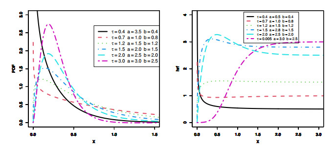
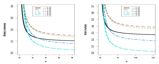
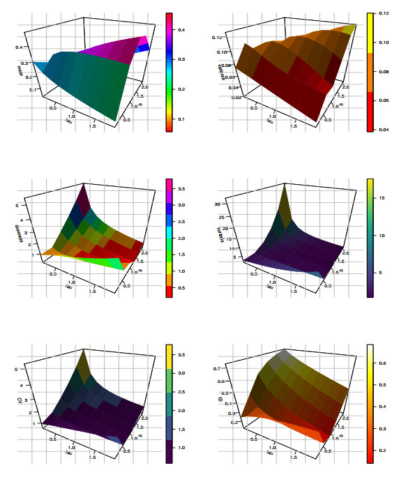
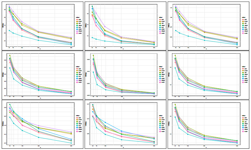
In this article, a new three-parameter lifetime model called the Gull alpha power exponentiated exponential (GAPEE) distribution is introduced and studied by combining the Gull alpha power family of distributions and the exponentiated exponential distribution. The shapes of the probability density function (PDF) for the GAPEE distribution can be asymmetric shapes, like unimodal, decreasing, and right-skewed. In addition, the shapes of the hazard rate function (hrf) for the GAPEE distribution can be increasing, decreasing, and upside-down shaped. Several statistical features of the GAPEE distribution are computed. Eight estimation methods such as the maximum likelihood, Anderson-Darling, right-tail Anderson-Darling, left-tailed Anderson-Darling, Cramér-von Mises, least-squares, weighted least-squares, and maximum product of spacing are discussed to estimate the parameters of the GAPEE distribution. The flexibility and the importance of the GAPEE distribution were demonstrated utilizing three real-world datasets related to medical sciences. The GAPEE distribution is extremely adaptable and outperforms several well-known statistical models. A bivariate step-stress accelerated life test based on progressive type-I censoring using the model is presented. Minimizing the asymptotic variance of the maximum likelihood estimate of the log of the scale parameter at design stress under progressive type-I censoring yields an expression for the ideal test plan under progressive type-I censoring.
- exponentiated exponential distribution,
- Gull alpha power family of distributions,
- bivariate step-stress,
- maximum likelihood estimation,
- progressive type-I censoring,
- symmetric,
- asymmetric,
- accelerated life test
Citation: Naif Alotaibi, A. S. Al-Moisheer, Ibrahim Elbatal, Salem A. Alyami, Ahmed M. Gemeay, Ehab M. Almetwally. Bivariate step-stress accelerated life test for a new three-parameter model under progressive censored schemes with application in medical[J]. AIMS Mathematics, 2024, 9(2): 3521-3558. doi: 10.3934/math.2024173

Related Papers:

Abstract

In this article, a new three-parameter lifetime model called the Gull alpha power exponentiated exponential (GAPEE) distribution is introduced and studied by combining the Gull alpha power family of distributions and the exponentiated exponential distribution. The shapes of the probability density function (PDF) for the GAPEE distribution can be asymmetric shapes, like unimodal, decreasing, and right-skewed. In addition, the shapes of the hazard rate function (hrf) for the GAPEE distribution can be increasing, decreasing, and upside-down shaped. Several statistical features of the GAPEE distribution are computed. Eight estimation methods such as the maximum likelihood, Anderson-Darling, right-tail Anderson-Darling, left-tailed Anderson-Darling, Cramér-von Mises, least-squares, weighted least-squares, and maximum product of spacing are discussed to estimate the parameters of the GAPEE distribution. The flexibility and the importance of the GAPEE distribution were demonstrated utilizing three real-world datasets related to medical sciences. The GAPEE distribution is extremely adaptable and outperforms several well-known statistical models. A bivariate step-stress accelerated life test based on progressive type-I censoring using the model is presented. Minimizing the asymptotic variance of the maximum likelihood estimate of the log of the scale parameter at design stress under progressive type-I censoring yields an expression for the ideal test plan under progressive type-I censoring.

References

[1]	M. M. Abdelwahab, A. B. Ghorbal, A. S. Hassan, M. Elgarhy, E. M. Almetwally, A. F. Hashem, Classical and bayesian inference for the Kavya-Manoharan generalized exponential distribution under generalized progressively hybrid censored data, Symmetry, 15 (2023). https://doi.org/10.3390/sym15061193
[2]	A. A. Alahmadi, M. Alqawba, W. Almutiry, A. W. Shawki, S. Alrajhi, S. Al-Marzouki, et al., A new version of weighted Weibull distribution: Modelling to COVID-19 data, Discrete Dyn. Nat. Soc., 2022 (2022). https://doi.org/10.1155/2022/3994361
[3]	Z. Ahmad, M. Elgarhy, G. Hamedani, N. S. Butt, Odd generalized NH generated family of distributions with application to exponential model, Pak. J. Stat. Oper. Res., 16 (2020), 53–71. https://doi.org/10.18187/pjsor.v16i1.2295 doi: 10.18187/pjsor.v16i1.2295
[4]	H. Al-Mofleh, M. Elgarhy, A. Afify, M. Zannon, Type II exponentiated half logistic generated family of distributions with applications, Electron. J. Appl. Stat., 13 (2020), 536–561.
[5]	A. M. Basheer, E. M. Almetwally, H. M. Okasha, Marshall-olkin alpha power inverse Weibull distribution: Non Bayesian and Bayesian estimations, J. Stat. Appl. Probab., 10 (2021), 327–345. https://doi.org/10.18576/jsap/100205 doi: 10.18576/jsap/100205
[6]	E. M. Almetwally, Marshall olkin alpha power extended Weibull distribution: Different methods of estimation based on type I and type II censoring, Gazi U. J. Sci., 35 (2022), 293–312. https://doi.org/10.35378/gujs.741755 doi: 10.35378/gujs.741755
[7]	E. M. Almetwally, The odd Weibull inverse Topp-Leone distribution with applications to COVID-19 data, Ann. Data Sci., 9 (2022), 121–140. https://doi.org/10.1007/s40745-021-00329-w doi: 10.1007/s40745-021-00329-w
[8]	N. Alotaibi, I. Elbatal, E. M. Almetwally, S. A. Alyami, A. S. Al-Moisheer, M. Elgarhy, Truncated Cauchy power Weibull-G class of distributions: Bayesian and non-Bayesian inference modelling for COVID-19 and carbon fiber data, Mathematics, 10 (2022). https://doi.org/10.3390/math10091565
[9]	N. Alotaibi, I. Elbatal, E. M. Almetwally, S. A. Alyami, A. Al-Moisheer, M. Elgarhy, Bivariate step-stress accelerated life tests for the Kavya-Manoharan exponentiated Weibull model under progressive censoring with applications, Symmetry, 14 (2022). https://doi.org/10.3390/sym14091791
[10]	R. Alotaibi, A. Al Mutairi, E. M. Almetwally, C. Park, H. Rezk, Optimal design for a bivariate step-stress accelerated life test with alpha power exponential distribution based on type-I progressive censored samples, Symmetry, 14 (2022). https://doi.org/10.3390/sym14040830
[11]	S. A. Alyami, I. Elbatal, N. Alotaibi, E. M. Almetwally, H. M. Okasha, M. Elgarhy, Topp-Leone modified Weibull model: Theory and applications to medical and engineering data, Appl. Sci., 12 (2022). https://doi.org/10.3390/app122010431
[12]	C. B. Ampadu, Gull Alpha power of the Ampadu-type: Properties and applications, Earthline J. Math. Sci., 6 (2021), 187–207. https://doi.org/10.34198/ejms.6121.187207 doi: 10.34198/ejms.6121.187207
[13]	T. W. Anderson, D. A. Darling, Asymptotic theory of certain "goodness of fit" criteria based on stochastic processes, Ann. Math. Stat., 23 (1952), 193–212. https://doi.org/10.1214/aoms/1177729437 doi: 10.1214/aoms/1177729437
[14]	J. M. Astorga, Y. A. Iriarte, H. W. Gómez, H. Bolfarine, Modified slashed generalized exponential distribution, Commun. Stat.-Theory M., 49 (2020), 4603–4617. https://doi.org/10.1080/03610926.2019.1604959 doi: 10.1080/03610926.2019.1604959
[15]	N. Balakrishnan, D. Han, G. Iliopoulos, Exact inference for progressively type-I censored exponential failure data, Metrika, 73 (2011), 335–358. https://doi.org/10.1007/s00184-009-0281-0 doi: 10.1007/s00184-009-0281-0
[16]	R. A. R. Bantan, C. Chesneau, F. Jamal, I. Elbatal, M. Elgarhy, The truncated burr XG family of distributions: Properties and applications to actuarial and financial data, Entropy, 23 (2021), 1088. https://doi.org/10.3390/e23081088 doi: 10.3390/e23081088
[17]	R. A. Bantan, F. Jamal, C. Chesneau, M. Elgarhy, On a new result on the ratio exponentiated general family of distributions with applications, Mathematics, 8 (2020), 598. https://doi.org/10.3390/math8040598 doi: 10.3390/math8040598
[18]	K. V. P. Barco, J. Mazucheli, V. Janeiro, The inverse power Lindley distribution, Commun. Stat.-Simul. C., 46 (2017), 6308–6323. https://doi.org/10.1080/03610918.2016.1202274 doi: 10.1080/03610918.2016.1202274
[19]	W. B. Souza, A. H. Santos, G. M. Cordeiro, The beta generalized exponential distribution, J. Stat. Comput. Sim., 80 (2010), 159–172. https://doi.org/10.1080/00949650802552402 doi: 10.1080/00949650802552402
[20]	M. Capanu, M. Giurcanu, C. B. Begg, M. Gönen, Subsampling based variable selection for generalized linear models, Comput. Stat. Data An., 184 (2023), 107740. https://doi.org/10.1016/j.csda.2023.107740 doi: 10.1016/j.csda.2023.107740
[21]	J. M. Carrasco, E. M. Ortega, G. M. Cordeiro, A generalized modified Weibull distribution for lifetime modeling, Computat. Stat. Data An., 53 (2008), 450–462. https://doi.org/10.1016/j.csda.2008.08.023 doi: 10.1016/j.csda.2008.08.023
[22]	A. K. Chaudhary, L. P. Sapkota, V. Kumar, Half-Cauchy generalized exponential distribution: Theory and application, J. Nepal Math. Soc., 5 (2022), 1–10. https://doi.org/10.3126/jnms.v5i2.50018 doi: 10.3126/jnms.v5i2.50018
[23]	K. Choi, W. G. Bulgren, An estimation procedure for mixtures of distributions, J. Roy. Stat. Soc. B, 30 (1968), 444–460. https://doi.org/10.1111/j.2517-6161.1968.tb00743.x doi: 10.1111/j.2517-6161.1968.tb00743.x
[24]	G. M. Cordeiro, E. M. Ortega, A. J. Lemonte, The exponential-Weibull lifetime distribution, J. Stat. Comput. Sim., 84 (2014), 2592–2606. https://doi.org/10.1080/00949655.2013.797982 doi: 10.1080/00949655.2013.797982
[25]	G. M. Cordeiro, E. M. Ortega, S. Nadarajah, The Kumaraswamy Weibull distribution with application to failure data, J. Franklin I., 347 (2010), 1399–1429. https://doi.org/10.1016/j.jfranklin.2010.06.010 doi: 10.1016/j.jfranklin.2010.06.010
[26]	G. M. Cordeiro, M. Alizadeh, G. Ozel, B. Hosseini, E. M. M. Ortega, E. Altun, The generalized odd log-logistic class of distributions: Properties, regression models and applications, J. Stat. Comput. Sim., 87 (2017), 908–932. https://doi.org/10.1080/00949655.2016.1238088 doi: 10.1080/00949655.2016.1238088
[27]	A. H. El-Bassiouny, N. F. Abdo, H. S. Shahen, Exponential Lomax distribution, Int. J. Comput. Appl., 121 (2015). https://doi.org/10.5120/21602-4713
[28]	E. A. ElSherpieny, E. M. Almetwally, The exponentiated generalized Alpha power family of distribution: Properties and applications, Pak. J. Stat. Oper. Res., 18 (2022), 349–367. https://doi.org/10.18187/pjsor.v18i2.3515 doi: 10.18187/pjsor.v18i2.3515
[29]	R. C. Gupta, P. L. Gupta, R. D. Gupta, Modeling failure time data by Lehman alternatives, Commun. Stat.-Theor. M., 27 (1998), 887–904. https://doi.org/10.1080/03610929808832134 doi: 10.1080/03610929808832134
[30]	N. Hakamipour, Approximated optimal design for a bivariate step-stress accelerated life test with generalized exponential distribution under type-I progressive censoring, Int. J. Qual. Reliab. Ma., 38 (2021), 1090–1115. https://doi.org/10.1108/IJQRM-05-2020-0150 doi: 10.1108/IJQRM-05-2020-0150
[31]	M. A. Haq, M. Elgarhy, S. Hashmi, The generalized odd Burr III family of distributions: Properties, applications and characterizations, J. Taibah Univ. Sci., 13 (2019), 961–971. https://doi.org/10.1080/16583655.2019.1666785 doi: 10.1080/16583655.2019.1666785
[32]	E. A. Hassan, M. Elgarhy, E. A. Eldessouky, O. H. M. Hassan, E. A. Amin, E. M. Almetwally, Different estimation methods for new probability distribution approach based on environmental and medical data, Axioms, 12 (2023), 220. https://doi.org/10.3390/axioms12020220 doi: 10.3390/axioms12020220
[33]	W. He, Z. Ahmad, A. Z. Afify, H. Goual, The arcsine exponentiated-X family: Validation and insurance application, Complexity, 20 (2020), 8394815. https://doi.org/10.1155/2020/8394815 doi: 10.1155/2020/8394815
[34]	M. Ijaz, S. M. A. Alamgir, M. Farooq, S. A. Khan, S. Manzoor, A Gull Alpha Power Weibull distribution with applications to real and simulated data, Plos One, 15 (2020). https://doi.org/10.1371/journal.pone.0233080
[35]	F. Jamal, M. A. Nasir, G. Ozel, M. Elgarhy, N. M. Khan, Generalized inverted Kumaraswamy generated family of distributions: Theory and applications, J. Appl. Stat., 46 (2019), 2927–2944. https://doi.org/10.1080/02664763.2019.1623867 doi: 10.1080/02664763.2019.1623867
[36]	F. Jamal, C. Chesneau, K. Aidi, The sine extended odd Fréchet-G family of distribution with applications to complete and censored data, Math. Slovaca, 71 (2021), 961–982. https://doi.org/10.1515/ms-2021-0033 doi: 10.1515/ms-2021-0033
[37]	J. H. K. Kao, Computer methods for estimating Weibull parameters in reliability studies, IRE T. Reliab. Qual. Contr., 1958, 15–22. https://doi.org/10.1109/IRE-PGRQC.1958.5007164
[38]	H. A. Khogeer, A. Alrumayh, M. M. Abd El-Raouf, M. Kilai, R. Aldallal, Exponentiated gull alpha exponential distribution with application to COVID-19 data, J. Math., 2022 (2022). https://doi.org/10.1155/2022/4255079
[39]	M. Kilai, G. A. Waititu, W. A. Kibira, H. M. Alshanbari, M. El-Morshedy, A new generalization of Gull Alpha Power family of distributions with application to modeling COVID-19 mortality rates, Results Phys., 36 (2022), 105339. https://doi.org/10.1016/j.rinp.2022.105339 doi: 10.1016/j.rinp.2022.105339
[40]	D. Kumar, U. Singh, S. K. Singh, A new distribution using sine function its application to bladder cancer patients data, J. Stat. Appl. Pro., 4 (2015), 417–427.
[41]	A. Mahdavi, D. Kundu, A new method for generating distributions with an application to exponential distribution, Commun. Stat.-Theor. M., 46 (2017), 6543–6557. https://doi.org/10.1080/03610926.2015.1130839 doi: 10.1080/03610926.2015.1130839
[42]	M. Kpangay, L. O. Odongo, G. O. Orwa, The Kumaraswamy-Gull Alpha Power Rayleigh distribution: Properties and application to HIV/AIDS data, Int. J. Sci. Res. Eng., 37 (2023), 431–442.
[43]	E. M. Almetwally, R. Alotaibi, H. Rezk, Estimation and prediction for Alpha-Power Weibull distribution based on hybrid censoring, Symmetry, 15 (2023), 1687. https://doi.org/10.3390/sym15091687 doi: 10.3390/sym15091687
[44]	G. S. Mudholkar, D. K. Srivastava, Exponentiated Weibull family for analyzing bathtub failure-rate data, IEEE T. Reliab., 42 (1993), 299–302. https://doi.org/10.1109/24.229504 doi: 10.1109/24.229504
[45]	G. S. Mudholkar, D. K. Srivastava, M. Freimer, The exponentiated Weibull family: A reanalysis of the bus-motor-failure data, Technometrics, 37 (1995), 436–445. https://doi.org/10.1080/00401706.1995.10484376 doi: 10.1080/00401706.1995.10484376
[46]	M. Muhammad, R. A. R. Bantan, L. Liu, C. Chesneau, M. H. Tahir, F. Jamal, et al., The truncated Burr XG family of distributions: Properties and applications to actuarial and financial data, Mathematics, 9 (2021), 2758. https://doi.org/10.3390/math9212758 doi: 10.3390/math9212758
[47]	M. S. Mukhtar, M. El-Morshedy, M. S. Eliwa, H. M. Yousof, Expanded Fréchet model: Mathematical properties, copula, different estimation methods, applications and validation testing, Mathematics, 8 (2020), 1949. https://doi.org/10.3390/math8111949 doi: 10.3390/math8111949
[48]	S. Nadarajah, The exponentiated exponential distribution: A survey, ASTA-Adv. Stat. Anal., 95 (2011), 219–251. https://doi.org/10.1007/s10182-011-0154-5 doi: 10.1007/s10182-011-0154-5
[49]	W. B. Nelson, Accelerated testing: Statistical models, test plans, and data analysis, John Wiley & Sons, 2009.
[50]	Z. M. Nofal, A. Z. Afify, H. M. Yousof, G. M. Cordeiro, The generalized transmuted-G family of distributions, Commun. Stat.-Theor. M., 46 (2017), 4119–4136. https://doi.org/10.1080/03610926.2015.1078478 doi: 10.1080/03610926.2015.1078478
[51]	A. H. Tolba, A. H. Muse, A. Fayomi, H. M. Baaqeel, E. M. Almetwally, The Gull Alpha Power Lomax distributions: Properties, simulation, and applications to modeling COVID-19 mortality rates, Plos One, 18 (2023). https://doi.org/10.1371/journal.pone.0283308
[52]	M. M. Ristic, D. Kundu, Marshall-Olkin generalized exponential distribution, J. Stat. Comput. Sim., 73 (2015), 317–333. https://doi.org/10.1007/s40300-014-0056-x doi: 10.1007/s40300-014-0056-x
[53]	T. Ruzgas, M. Lukauskas, G. Čepkauskas, Nonparametric multivariate density estimation: Case study of Cauchy mixture model, Mathematics, 9 (2021), 2717. https://doi.org/10.3390/math9212717 doi: 10.3390/math9212717
[54]	L. P. Sapkota, V. Kumar, Odd lomax generalized exponential distribution: Application to engineering and COVID-19 data, Pak. J. Stat. Oper. Res., 18 (2022), 883–900. https://doi.org/10.18187/pjsor.v18i4.4149 doi: 10.18187/pjsor.v18i4.4149
[55]	D. C. U. Sivakumar, R. Kanaparthi, G. S. Rao, K. Kalyani, The odd generalized exponential log-logistic distribution group acceptance sampling plan, Stat. Transition New Series, 20 (2019), 103–116. https://doi.org/10.21307/stattrans-2019-006 doi: 10.21307/stattrans-2019-006
[56]	L. Souza, W. Junior, C. de Brito, C. Chesneau, R. Fernandes, T. Ferreira, Tan-G class of trigonometric distributions and its applications, Cubo, 23 (2021), 1–20. https://doi.org/10.4067/S0719-06462021000100001 doi: 10.4067/S0719-06462021000100001
[57]	L. Souza, W. R. O. Junior, C. C. R. de Brito, C. Chesneau, T. A. E. Ferreira, L. Soares, General properties for the Cos-G class of distributions with applications, Eurasian Bull. Math., 2 (2019), 63–79.
[58]	J. J. Swain, S. Venkatraman, J. R. Wilson, Least-squares estimation of distribution functions in Johnson's translation system, J. Stat. Comput. Sim., 29 (1988), 271–297. https://doi.org/10.1080/00949658808811068 doi: 10.1080/00949658808811068
[59]	H. Torabi, N. H. Montazeri, The logistic-uniform distribution and its application, Commun. Stat.-Simul. C., 43 (2014), 2551–2569. https://doi.org/10.1080/03610918.2012.737491 doi: 10.1080/03610918.2012.737491
[60]	X. Romao, R. Delgado, A. Costa, An empirical power comparison of univariate goodness-of-fit tests for normality, J. Stat. Computat. Sim., 80 (2010), 545–591. https://doi.org/10.1080/00949650902740824 doi: 10.1080/00949650902740824
[61]	R. A. ZeinEldin, C. Chesneau, F. Jamal, M. Elgarhy, A. M. Almarashi, S. Al-Marzouki, Generalized truncated Fréchet generated family distributions and their applications, CMES-Comp. Model. Eng., 126 (2021), 791–819. https://doi.org/10.32604/cmes.2021.012169 doi: 10.32604/cmes.2021.012169
[62]	C. Zhao, R. Zhuang, Statistical solutions and Liouville theorem for the second order lattice systems with varying coefficients, J. Differ. Equations, 372 (2023), 194–234. https://doi.org/10.1016/j.jde.2023.06.040 doi: 10.1016/j.jde.2023.06.040
[63]	S. Zhou, A. Xu, Y. Tang, L. Shen, Fast Bayesian inference of reparameterized Gamma process with random effects, IEEE T. Reliab., 2023 (2023) 1–14. https://doi.org/10.1109/TR.2023.3263940

Reader Comments

Your name:*

Email:*
© 2024 the Author(s), licensee AIMS Press. This is an open access article distributed under the terms of the Creative Commons Attribution License (http://creativecommons.org/licenses/by/4.0)