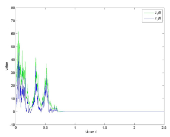
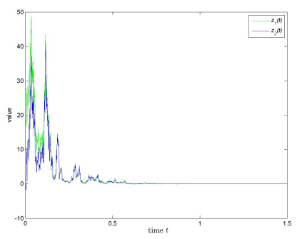
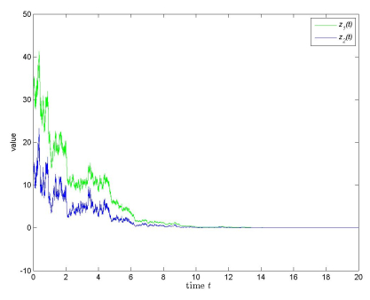
This paper centers on stochastic Hopfield neural networks with variable coefficients and infinite delay. First, we propose an integral inequality that improves and extends some existing works. Second, by employing some inequalities and stochastic analysis techniques, some sufficient conditions for ensuring $ p $th moment generalized exponential stability are established. Our results do not necessitate the construction of a complex Lyapunov function or rely on the assumption of bounded variable coefficients, and our results expand some existing works. At last, to illustrate the efficacy of our result, we present several simulation examples.
Citation: Dehao Ruan, Yao Lu. Generalized exponential stability of stochastic Hopfield neural networks with variable coefficients and infinite delay[J]. AIMS Mathematics, 2024, 9(8): 22910-22926. doi: 10.3934/math.20241114
This paper centers on stochastic Hopfield neural networks with variable coefficients and infinite delay. First, we propose an integral inequality that improves and extends some existing works. Second, by employing some inequalities and stochastic analysis techniques, some sufficient conditions for ensuring $ p $th moment generalized exponential stability are established. Our results do not necessitate the construction of a complex Lyapunov function or rely on the assumption of bounded variable coefficients, and our results expand some existing works. At last, to illustrate the efficacy of our result, we present several simulation examples.

| [1] |
T. Deb, A. K. Ghosh, A. Mukherjee, Singular value decomposition applied to associative memory of Hopfield neural network, Mater. Today: Proc., 5 (2018), 2222–2228. https://doi.org/10.1016/j.matpr.2017.09.222 doi: 10.1016/j.matpr.2017.09.222

|
| [2] |
M. Muneyasu, K. Yamamoto, T. Hinamoto, Image restoration using layered neural networks and Hopfield networks, Proceedings., International Conference on Image Processing, 2 (1995), 33–36. https://doi.org/10.1109/ICIP.1995.537408 doi: 10.1109/ICIP.1995.537408
|
| [3] |
P. N. Suganthan, E. K. Teoh, D. P. Mital, Pattern recognition by homomorphic graph matching using Hopfield neural networks, Image Vision Comput., 13 (2015), 45–60. https://doi.org/10.1016/0262-8856(95)91467-R doi: 10.1016/0262-8856(95)91467-R
|
| [4] |
C. M. Marcus, R. M. Westervelt, Stability of analog neural networks with delay, Phys. Rev. A, 39 (1989), 347–359. https://doi.org/10.1103/physreva.39.347 doi: 10.1103/physreva.39.347
|
| [5] |
X. Wang, M. Jiang, S. Fang, Stability analysis in Lagrange sense for a non-autonomous Cohen-Grossberg neural network with mixed delays, Nonlinear Anal.: Theory Methods Appl., 70 (2009), 4294–4306. https://doi.org/10.1016/j.na.2008.09.019 doi: 10.1016/j.na.2008.09.019
|
| [6] | S. Haykin, Neural networks: a comprehensive foundation, 3 Eds., Prentice-Hall, Inc., 2007. |
| [7] |
Z. Wang, H. Shu, J. Fang, X. Liu, Robust stability for stochastic Hopfield neural networks with time delays, Nonlinear Anal.: Real World Appl., 7 (2006), 1119–1128. https://doi.org/10.1016/j.nonrwa.2005.10.004 doi: 10.1016/j.nonrwa.2005.10.004
|
| [8] |
Z. Wang, Y. Liu, K. Fraser, X. Liu, Stochastic stability of uncertain Hopfield neural networks with discrete and distributed delays, Phys. Lett. A, 354 (2006), 288–297. https://doi.org/10.1016/j.physleta.2006.01.061 doi: 10.1016/j.physleta.2006.01.061
|
| [9] |
Y. Chen, Z. Wang, Y. Liu, F. E. Alsaadi, Stochastic stability for distributed delay neural networks via augmented Lyapunov-Krasovskii functionals, Appl. Math. Comput., 338 (2018), 869–881. https://doi.org/10.1016/j.amc.2018.05.059 doi: 10.1016/j.amc.2018.05.059
|
| [10] |
Q. Zhou, L. Wan, Exponential stability of stochastic delayed Hopfield neural networks, Appl. Math. Comput., 199 (2008), 84–89. https://doi.org/10.1016/j.amc.2007.09.025 doi: 10.1016/j.amc.2007.09.025
|
| [11] |
J. Hu, S. Zhong, L. Liang, Exponential stability analysis of stochastic delayed cellular neural network, Chaos Soliton. Fract., 27 (2006), 1006–1010. https://doi.org/10.1016/j.chaos.2005.04.067 doi: 10.1016/j.chaos.2005.04.067
|
| [12] |
L. Liu, F. Deng, Stability analysis of time varying delayed stochastic Hopfield neural networks in numerical simulation, Neurocomputing, 316 (2018), 294–305. https://doi.org/10.1016/j.neucom.2018.08.004 doi: 10.1016/j.neucom.2018.08.004
|
| [13] |
J. Luo, Fixed points and stability of neutral stochastic delay differential equations, J. Math. Anal. Appl., 334 (2007), 431–440. https://doi.org/10.1016/j.jmaa.2006.12.058 doi: 10.1016/j.jmaa.2006.12.058
|
| [14] |
J. Luo, Fixed points and exponential stability of mild solutions of stochastic partial differential equations with delays, J. Math. Anal. Appl., 342 (2008), 753–760. https://doi.org/10.1016/j.jmaa.2007.11.019 doi: 10.1016/j.jmaa.2007.11.019
|
| [15] |
J. Luo, Fixed points and exponential stability for stochastic Volterra-Levin equations, J. Comput. Appl. Math., 234 (2010), 934–940. https://doi.org/10.1016/j.cam.2010.02.013 doi: 10.1016/j.cam.2010.02.013
|
| [16] |
G. Chen, D. Li, L. Shi, O. van Ganns, S. V. Lunel, Stability results for stochastic delayed recurrent neural networks with discrete and distributed delays, J. Differ. Equations, 264 (2018), 3864–3898. https://doi.org/10.1016/j.jde.2017.11.032 doi: 10.1016/j.jde.2017.11.032
|
| [17] |
Q. Song, R. Zeng, Z. Zhao, Y. Liu, F. E. Alsaadi, Mean-square stability of stochastic quaternion-valued neural networks with variable coefficients and neutral delays, Neurocomputing, 471 (2022), 130–138. https://doi.org/10.1016/j.neucom.2021.11.033 doi: 10.1016/j.neucom.2021.11.033
|
| [18] |
X. Hou, H. Wu, J. Cao, Observer-based prescribed-time synchronization and topology identification for complex networks of piecewise-smooth systems with hybrid impulses, Comput. Appl. Math., 43 (2008), 180. https://doi.org/10.1007/s40314-024-02701-x doi: 10.1007/s40314-024-02701-x
|
| [19] |
Y. Zhao, H. Wu, Fixed/Prescribed stability criterions of stochastic system with time-delay, AIMS Math., 9 (2024), 14425–14453. https://doi.org/10.3934/math.2024701 doi: 10.3934/math.2024701
|
| [20] |
L. Wan, J. Sun, Mean square exponential stability of stochastic delayed Hopfield neural networks, Phys. Lett. A, 343 (2005), 306–318. https://doi.org/10.1016/j.physleta.2005.06.024 doi: 10.1016/j.physleta.2005.06.024
|
| [21] |
Y. Sun, J. Cao, $p$th moment exponential stability of stochastic recurrent neural networks with time-varying delays, Nonlinear Anal.: Real World Appl., 8 (2007), 1171–1185. https://doi.org/10.1016/j.nonrwa.2006.06.009 doi: 10.1016/j.nonrwa.2006.06.009
|
| [22] |
X. Li, D. Deng, Mean square exponential stability of stochastic Hopfield neural networks with mixed delays, Stat. Probab. Lett., 126 (2017), 88–96. https://doi.org/10.1016/j.spl.2017.02.029 doi: 10.1016/j.spl.2017.02.029
|
| [23] |
D. Ruan, Z. Huang, X. Guo, Inequalities and stability of stochastic Hopfield neural networks with discrete and distributed delays, Neurocomputing, 407 (2020), 281–291. https://doi.org/10.1016/j.neucom.2020.05.005 doi: 10.1016/j.neucom.2020.05.005
|
| [24] |
F. Zhang, C. Fei, W. Fei, Stability of stochastic Hopfield neural networks driven by $G$-Brownian motion with time-varying and distributed delays, Neurocomputing, 520 (2023), 320–330. https://doi.org/10.1016/j.neucom.2022.10.065 doi: 10.1016/j.neucom.2022.10.065
|
| [25] |
B. Lu, H. Jiang, A. Abdurahman, C. Hu, Global generalized exponential stability for a class of nonautonomous cellular neural networks via generalized Halanay inequalities, Neurocomputing, 214 (2016), 1046–1052. https://doi.org/10.1016/j.neucom.2016.06.068 doi: 10.1016/j.neucom.2016.06.068
|
| [26] |
C. Huang, Y. He, H. Wang, Mean square exponential stability of stochastic recurrent neural networks with time-varying delays, Comput. Math. Appl., 56 (2008), 1773–1778. https://doi.org/10.1016/j.camwa.2008.04.004 doi: 10.1016/j.camwa.2008.04.004
|
| [27] |
C. Huang, Y. He, L. Huang, W. Zhu, $p$th moment stability analysis of stochastic recurrent neural networks with time-varying delays, Inf. Sci., 178 (2008), 2194–2203. https://doi.org/10.1016/j.ins.2008.01.008 doi: 10.1016/j.ins.2008.01.008
|
| [28] |
X. Lai, Y. Zhang, Fixed point and asymptotic analysis of cellular neural networks, J. Appl. Math., 2012 (2012), 701–708. https://doi.org/10.1155/2012/689845 doi: 10.1155/2012/689845
|
| [29] | R. A. Horn, C. R. Johnson, Matrix analysis, Cambridge University Press, 1985. https://doi.org/10.1017/CBO9780511810817 |
| [30] | A. Friedman, Stochastic differential equations and applications, In: J. Cecconi, Stochastic differential equations, C.I.M.E. Summer Schools, Springer, 77 (1997), 75–148. https://doi.org/10.1007/978-3-642-11079-5_2 |
Figures(3)

Dehao Ruan, Yao Lu. Generalized exponential stability of stochastic Hopfield neural networks with variable coefficients and infinite delay[J]. AIMS Mathematics, 2024, 9(8): 22910-22926. doi: 10.3934/math.20241114


 DownLoad: