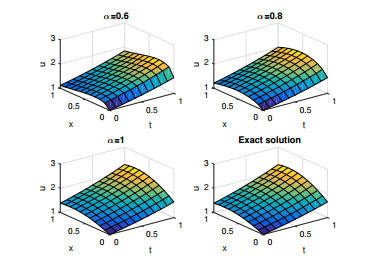
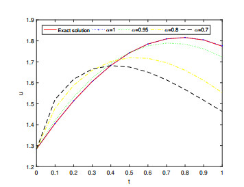
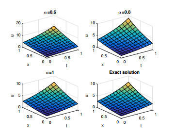
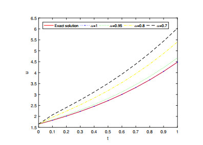
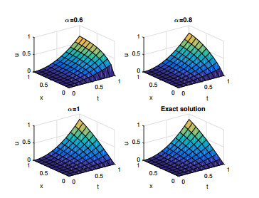
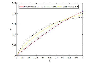
The main purpose of this paper is to present a new computational for approximate analytical solutions of nonlinear time-fractional wave-like equations with variable coefficients using the fractional residual power series method (FRPSM). The fractional derivative is considered in the Caputo sense. This method is based on the generalized Taylor series formula and residual error function. Unlike other analytical methods, FRPSM has a special advantage, that it solves the nonlinear problems without using linearization, discretization, perturbation or any other restrictions. By numerical examples, it is shown that the FRPSM is a simple, effective, and powerful method for finding approximate analytical solutions of nonlinear fractional partial differential equations.
Citation: Ali Khalouta, Abdelouahab Kadem. A new computational for approximate analytical solutions of nonlinear time-fractional wave-like equations with variable coefficients[J]. AIMS Mathematics, 2020, 5(1): 1-14. doi: 10.3934/math.2020001
The main purpose of this paper is to present a new computational for approximate analytical solutions of nonlinear time-fractional wave-like equations with variable coefficients using the fractional residual power series method (FRPSM). The fractional derivative is considered in the Caputo sense. This method is based on the generalized Taylor series formula and residual error function. Unlike other analytical methods, FRPSM has a special advantage, that it solves the nonlinear problems without using linearization, discretization, perturbation or any other restrictions. By numerical examples, it is shown that the FRPSM is a simple, effective, and powerful method for finding approximate analytical solutions of nonlinear fractional partial differential equations.

| [1] |
O. Abu Arqub, Series solution of fuzzy differential equations under strongly generalized differentiability, J. Adv. Res. Appl. Math., 5 (2013), 31-52. doi: 10.5373/jaram.1447.051912

|
| [2] |
O. Acan, M. M. Al Qurashi and D. Baleanu, Reduced differential transform method for solving time and space local fractional partial differential equations, J. Nonlinear Sci. Appl., 10 (2017), 5230-5238. doi: 10.22436/jnsa.010.10.09
|
| [3] | M. Dehghan, J. Manafian and A. Saadatmandi, Solving nonlinear fractional partial differential equations using the homotopy analysis method, Numer. Meth. Part. D. E., 26 (2009), 448-479. |
| [4] |
A. El-Ajou, O. Abu Arqub, Z. Al Zhour, et al. New results on fractional power series: theories and applications, Entropy, 15 (2013), 5305-5323. doi: 10.3390/e15125305
|
| [5] |
A. El-Ajou, O. AbuArquba and Sh. Momanib, Approximate analytical solution of the nonlinear fractional KdV-Burgers equation: A new iterative algorithm, J. Comput. Phys., 293 (2015), 81-95. doi: 10.1016/j.jcp.2014.08.004
|
| [6] |
A. Elsaid, The variational iteration method for solving Riesz fractional partial differential equations, Comput. Math. Appl., 60 (2010), 1940-1947. doi: 10.1016/j.camwa.2010.07.027
|
| [7] |
A. A. Freihet and M. Zuriqat, Analytical Solution of Fractional Burgers-Huxley Equations via Residual Power Series Method, Lobachevskii Journal of Mathematics, 40 (2019), 174-182. doi: 10.1134/S1995080219020082
|
| [8] |
P. K. Gupta and M. Singh, Homotopy perturbation method for fractional Fornberg-Whitham equation, Comput. Math. Appl., 61 (2011), 250-254. doi: 10.1016/j.camwa.2010.10.045
|
| [9] | K. Hosseini, A. Bekir, M. Kaplan, et al. On On a new technique for solving the nonlinear conformable time-fractional differential equations, Opt. Quant. Electron., 49 (2017), 343. |
| [10] | M. Kaplan, A. Bekir, A. Akbulut, et al. The modified simple equation method for nonlinear fractional differential equations, Rom. J. Phys., 60 (2015), 1374-1383. |
| [11] |
M. Kaplan and A. Bekir, Construction of exact solutions to the space-time fractional differential equations via new approach, Optik, 132 (2017), 1-8. doi: 10.1016/j.ijleo.2016.11.139
|
| [12] | A. Khalouta and A. Kadem, Comparison of New Iterative Method and Natural Homotopy Perturbation Method for Solving Nonlinear Time-Fractional Wave-Like Equations with Variable Coefficients, Nonlinear Dyn. Syst. Theory, 19 (2019), 160-169. |
| [13] |
A. Khalouta and A. Kadem, Fractional natural decomposition method for solving a certain class of nonlinear time-fractional wave-like equations with variable coefficients, Acta Universitatis Sapientiae: Mathematica, 11 (2019), 99-116. doi: 10.2478/ausm-2019-0009
|
| [14] | A. Khalouta and A. Kadem, A New Technique for Finding Exact Solutions of Nonlinear TimeFractional Wave-Like Equations with Variable Coefficients, Proc. Inst. Math. Mech. Natl. Acad.Sci. Azerb., 2019. |
| [15] | A. Khalouta and A. Kadem, A New iterative natural transform method for solving nonlinear Caputo time-fractional partial differential equations, Appear in: Jordan J. Math. Stat., 2019. |
| [16] | A. Kilbas, H. M. Srivastava and J. J. Trujillo, Theory and Application of Fractional Differential equations, Elsevier, Amsterdam, 2006. |
| [17] |
A. Kumar, S. Kumar and M. Singh, Residual power series method for fractional Sharma-TassoOlever equation, Commun. Numer. Anal., 2016 (2016), 1-10. doi: 10.5899/2016/cna-00235
|
| [18] | K. S. Miller and B. Ross, An Introduction to the Fractional Calculus and Fractional Differential Equations, John Willey and Sons, New York, 1993. |
| [19] | Z. Pinar, On the explicit solutions of fractional Bagley-Torvik equation arises in engineering, An International Journal of Optimization and Control: Theories & Applications (IJOCTA), 9 (2019), 52-58. |
| [20] | I. Podlubny, Fractional Differential Equations, Academic Press, New York, 1999. |
| [21] | F. Tchier, M. Inc, Z. S. Korpinar, et al. Solutions of the time fractional reaction-diffusion equations with residual power series method, Adv. Mech. Eng., 8 (2016), 1-10. |
| [22] | H. Thabet and S. Kendre, New modification of Adomian decomposition method for solving a system of nonlinear fractional partial differential equations, Int. J. Adv. Appl. Math. and Mech., 6 (2019), 1-13. |
| [23] |
S. Uçar, E. Uçar, N. Özdemira, et al. Mathematical analysis and numerical simulation for a smoking model with Atangana-Baleanu derivative, Chaos Solitons Fractals, 118 (2019), 300-306. doi: 10.1016/j.chaos.2018.12.003
|
| [24] | M. Yavuz, Novel solution methods for initial boundary value problems of fractional order with conformable differentiation, An International Journal of Optimization and Control: Theories & Applications (IJOCTA), 8 (2017), 1-7. |
| [25] | M. Yavuz and N. Özdemira, Comparing the new fractional derivative operators involving exponential and Mittag-Leffler kernel, Discrete Contin. Dyn. Syst. Ser. S, 13 (2020), 995-1006. |
Figures(6) / Tables(3)

Ali Khalouta, Abdelouahab Kadem. A new computational for approximate analytical solutions of nonlinear time-fractional wave-like equations with variable coefficients[J]. AIMS Mathematics, 2020, 5(1): 1-14. doi: 10.3934/math.2020001


 DownLoad: