Geotechnical characterization of Halsen-Stjørdal silt, Norway

Annika Bihs; Mike Long; Steinar Nordal; Annika Bihs; Mike Long; Steinar Nordal

doi:10.3934/geosci.2020020

AIMS Geosciences

2020, Volume 6, Issue 3: 355-377. doi: 10.3934/geosci.2020020

Previous Article Next Article

Research article

Geotechnical characterization of Halsen-Stjørdal silt, Norway

1.
Department of Civil and Environmental Engineering, Norwegian University of Science and Technology (NTNU), 7491 Trondheim, Norway
2.
School of Civil Engineering, University College Dublin (UCD), Newstead Building Belfield, Dublin 4, Ireland

Received: 13 August 2020 Accepted: 16 September 2020 Published: 21 September 2020

The evaluation of geotechnical parameters for design problems in silty soils is complicated due to partially drained conditions and irregular soil structure, including small layers and pockets of both coarser and finer material. Many established methods to define soil parameters in clay and sand exist but little guidance is given to practicing engineers on how to interpret soil parameters for silty materials. This paper presents the results of an extensive laboratory and field test program which was carried out at a silt testing site Halsen-Stjø rdal in Norway. The main objective is to broaden the database of the engineering behaviour of silts and to gain a better understanding of the behaviour of these soils. Cone penetration tests (CPTU) were performed and shear wave velocity measurements close to the site were used to supplement the CPTU results, confirming the coarse, silty nature of the deposit. In addition, several samples were taken using thin walled 54 mm steel sample tubes and examined in the laboratory by means of index, oedometer and triaxial tests. Recently developed methods to determine sample quality in intermediate low plastic soils were adopted and showed promising results. The interpretation of the oedometer tests was challenging due to the shapes of the curves. The results did not identify the yield or preconsolidation stress clearly partly due to the nature of the silt and partly due to sample disturbance. Triaxial test results on the silt showed a strong dilative behaviour developing negative pore pressures with increasing axial strain. The shape of the stress paths revealed no unique undrained shear strength of the silt. Although many researchers doubt the use of undrained shear strength (s_u) for partially drained materials, this parameter is still frequently used. Several methods were applied to determine values of an apparent s_u in the silt in order to provide an overview over the range of strength values. The results from this study contribute to the existing database and increase the understanding of silty soils.
- silt,
- CPTU,
- laboratory test,
- drainage,
- sample quality
Citation: Annika Bihs, Mike Long, Steinar Nordal. Geotechnical characterization of Halsen-Stjørdal silt, Norway[J]. AIMS Geosciences, 2020, 6(3): 355-377. doi: 10.3934/geosci.2020020

Related Papers:

Abstract

The evaluation of geotechnical parameters for design problems in silty soils is complicated due to partially drained conditions and irregular soil structure, including small layers and pockets of both coarser and finer material. Many established methods to define soil parameters in clay and sand exist but little guidance is given to practicing engineers on how to interpret soil parameters for silty materials. This paper presents the results of an extensive laboratory and field test program which was carried out at a silt testing site Halsen-Stjø rdal in Norway. The main objective is to broaden the database of the engineering behaviour of silts and to gain a better understanding of the behaviour of these soils. Cone penetration tests (CPTU) were performed and shear wave velocity measurements close to the site were used to supplement the CPTU results, confirming the coarse, silty nature of the deposit. In addition, several samples were taken using thin walled 54 mm steel sample tubes and examined in the laboratory by means of index, oedometer and triaxial tests. Recently developed methods to determine sample quality in intermediate low plastic soils were adopted and showed promising results. The interpretation of the oedometer tests was challenging due to the shapes of the curves. The results did not identify the yield or preconsolidation stress clearly partly due to the nature of the silt and partly due to sample disturbance. Triaxial test results on the silt showed a strong dilative behaviour developing negative pore pressures with increasing axial strain. The shape of the stress paths revealed no unique undrained shear strength of the silt. Although many researchers doubt the use of undrained shear strength (s_u) for partially drained materials, this parameter is still frequently used. Several methods were applied to determine values of an apparent s_u in the silt in order to provide an overview over the range of strength values. The results from this study contribute to the existing database and increase the understanding of silty soils.

References

[1]	Senneset K, Sandven R, Janbu N (1989) Evaluation of soil parameters from piezocone tests. Transp Res Rec, 24-37.
[2]	Long M, Gudjonsson G, Donohue S, et al. (2010) Engineering characterisation of Norwegian glaciomarine silt. Eng Geol 110: 51-65. doi: 10.1016/j.enggeo.2009.11.002
[3]	Blaker Ø , Carroll R, Paniagua P, et al. (2019) Halden research site: geotechnical characterization of a post glacial silt. AIMS Geosci 5: 184-234. doi: 10.3934/geosci.2019.2.184
[4]	Lunne T, Berre T, Strandvik S (1997) Sample disturbance effects in soft low plastic Norwegian clay. In: Recent Developments in Soil and Pavement Mechanics. Rio de Janeiro, Brazil: Balkema, 81-102.
[5]	Andresen A, Kolstad P (1979) The NGI 54 mm sampler for undisturbed sampling of clays and representative sampling of coarse materials. In: International Symposium on soil sampling. Singapore, 13-21.
[6]	DeJong JT, Krage CP, Albin BM, et al. (2018) Work-Based Framework for Sample Quality Evaluation of Low Plasticity Soils. J Geotech Geoenviron Eng 144: 04018074. doi: 10.1061/(ASCE)GT.1943-5606.0001941
[7]	Janbu N (1963) Soil compressibility as determined by odometer and triaxial tests. In: 3rd European Conference on Soil Mechanics and Foundation Engineering. Wiesbaden, Germany, 19-25.
[8]	Becker DE, Crooks JHA, Been K, et al. (1987) Work as a criterion for determining in situ and yield stresses in clays. Can Geotech J 24: 549-564. doi: 10.1139/t87-070
[9]	Brandon TL, Rose AT, Duncan JM (2006) Drained and Undrained Strength Interpretation for Low-Plasticity Silts. J Geotech Geoenviron Eng 132: 250-257. doi: 10.1061/(ASCE)1090-0241(2006)132:2(250)
[10]	Schneider J, Randolph M, Mayne P, et al. (2008) Analysis of Factors Influencing Soil Classification Using Normalized Piezocone Tip Resistance and Pore Pressure Parameters. J Geotech Geoenviron Eng 134: 1569-1586. doi: 10.1061/(ASCE)1090-0241(2008)134:11(1569)
[11]	Robertson P (1990) Soil classification using the cone penetration test. Can Geotech J 27: 151-158. doi: 10.1139/t90-014
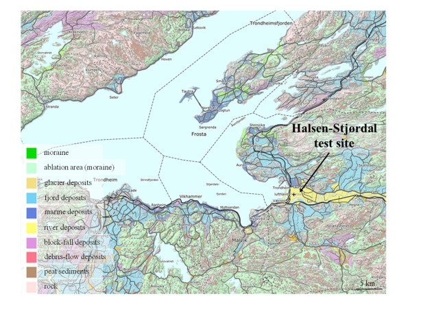
[12]	Sveian H (1995) Sandsletten blir til: Stjø rdal fra fjordbunn til strandsted. Trondheim: Norges Geologiske Undersø kelse (NGU).
[13]	NGU (2020) Superficial deposits—National Database, Geological Survey of Norway (NGU). Available from: http://geo.ngu.no/kart/losmasse_mobil/?lang=eng.
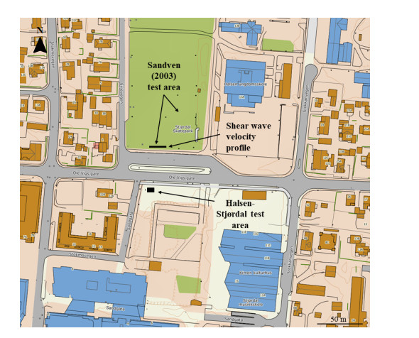
[14]	Sandven R (2003) Geotechnical properties of a natural silt deposit obtained from field and laboratory tests. In: International Workshop on characterization and engineering properties of natural soils. Singapore: Balkema, 1121-1148.
[15]	Lunne T, Robertson PK, Powell JJM (1997) Cone Penetration Testing in Geotechnical Practice: Blackie Academic and Professional.
[16]	Amundsen HA, Thakur V (2018) Storage Duration Effects on Soft Clay Samples. Geotech Test J 42: 1031-1054.
[17]	NGU (2020) Arealinformasjon—Norge og Svalbard med havområ der, Geological Survey of Norway (NGU). Available from: http://geo.ngu.no/kart/arealis_mobil/?extent=296823,7044369,297380,7044631.
[18]	ISO (2012) Geotechnical investigation and testing—Field testing. Part I: Electrical cone and piezocone penetration test. Geneva, Switzerland: International Organization for Standardization (ISO).
[19]	Senneset K, Janbu N (1985) Shear strength parameters obtained from static cone penetration tests. In: ASTM Speciality Conference, Strength Testing of Marine Sediments, Laboratory and In Situ Measurements. San Diego, 41-54.
[20]	Robertson P, Campanella RG, Gillespie D, et al. (1986) Use of piezometer cone data. In: ASCE Speciality Conference In Situ '86: Use of In Situ Tests in Geotechnical Engineering. Blacksburg, 1263-1280.
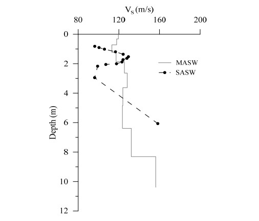
[21]	Nazarian S, Stokoe KH (1984) In situ shear wave velocities from spectral analysis of surface waves. 8th World Conference on Earthquake Engineering. San Francisco, 31-38.
[22]	Park CB, Miller DM, Xia J (1999) Multichannel analysis of surface waves. Geophysics 64: 800-808. doi: 10.1190/1.1444590
[23]	Heisey JS, Stokoe KH, Meyer AH (1982) Moduli of pavement systems for spectral analysis of surface waves. In: 61^st Annual Meeting of the Transportation Research Boad. Washington, D.C., 22-31.
[24]	NIBS (2003) National Earthquake Hazard Reduction Program (NEHRP)—Recommended provisions for seismic regulations for new buildings and other structures (FEMA 450) Part 1: Provisions. Building Seismic Safety Council of the National Instiute of Building Sciences (NIBS). Washington, D.C.
[25]	Lunne T, Long M, Forsberg CF (2003) Characterization and engineering properties of Holmen, Drammen sand. Characterisation and Engineering Properties of Natural Soils. Singapore, 1121-1148.
[26]	NGF (2013) Melding 11: Veiledning for prø vetaking (in Norwegian). Oslo, Norway: Norwegian Geotechnical Society (NGF).
[27]	Terzaghi K, Peck RB, Mesri G (1996) Soil Mechanics in Engineering Practice. John Wiley and Sons.
[28]	Lunne T, Berre T, Andersen KH, et al. (2006) Effects of sample disturbance and consolidation procedures on measured shear strength of soft marine Norwegian clays. Can Geotech J 43: 726-750. doi: 10.1139/t06-040
[29]	Long M, Sandven R, Gudjonsson GT (2005) Parameterbestemmelser for siltige materialer. Delrapport C (in Norwegian). Statens Vegvesen.
[30]	Carroll R, Long M (2017) Sample Disturbance Effects in Silt. J Geotech Geoenviron Eng 143: 04017061. doi: 10.1061/(ASCE)GT.1943-5606.0001749
[31]	Donohue S, Long M (2010) Assessment of sample quality in soft clay using shear wave velocity and suction measurements. Géotechnique 60: 883-889. doi: 10.1680/geot.8.T.007.3741
[32]	Donohue S, Long M (2007) Rapid Determination of Soil Sample Quality Using Shear Wave Velocity And Suction Measurements. In: 6th International Offshore Site Investigation and Geotechnics Conference: Society for Underwater Technology, 63-72.
[33]	Krage C, Albin B, Dejong JT, et al. (2016) The Influence of In-situ Effective Stress on Sample Quality for Intermediate Soils. In: Geotechnical and Geophysical Site Characterization 5-ISC5. Gold Coast, Australia, 565-570.
[34]	Amundsen HA (2018) Storage duration effects on Norwegian low-plasticity sensitive clay samples. Trondheim: Norwegian University of Science and Technology (NTNU).
[35]	NGF (2011) Melding 2: Veiledning for symboler og definisjoner i geoteknikk—identifisering og klassifisering av jord (in Norwegian): Norwegian Geotechnical Society (NGF).
[36]	Bihs A, Nordal S, Long M, et al. (2018) Effect of piezocone penetration rate on the classification of Norwegian silt. In: Cone Penetration Testing 2018 (CPT'18), CRC Press/Balkema.
[37]	Sandbaekken G, Berre T, Lacasse S (1986) Oedometer Testing at the Norwegian Geotechnical Institute. In: Yong RN, Townsend FC, editors, Consolidation of Soils: Testing and Evaluation. West Conshohocken, PA: ASTM, 329-353.
[38]	Boone SJ (2010) A critical reappraisal of "preconsolidation pressure" interpretations using the oedometer test. Can Geotech J 47: 281-296. doi: 10.1139/T09-093
[39]	Cola S, Simonini P (2002) Mechanical behavior of silty soils of the Venice lagoon as a function of their grading characteristics. Can Geotech J 39: 879-893. doi: 10.1139/t02-037
[40]	Shipton B, Coop MR (2012) On the compression behaviour of reconstituted soils. Soils Found 52: 668-681. doi: 10.1016/j.sandf.2012.07.008
[41]	Janbu N (1985) 25^th Rankine Lecture: Soil models in offshore engineering. Géotechnique 35: 241-281. doi: 10.1680/geot.1985.35.3.241
[42]	Senneset K, Sandven R, Lunne T, et al. (1988) Piezocone tests in silty soils. ISOPT-1. Orlando: Balkema, 955-966.
[43]	Sandven R (1990) Strength and deformation properties of fine grained soils obtained from piezocone tests. Trondheim, Norway: Norwegian University of Science and Technology (NTNU).
[44]	Casagrande A (1936) The determination of pre-consolidation load and it's practical significance. In: 1^st International Soil Mechanics and Foundation Engineering Conference. Cambridge, Massachusetts, 60-64.
[45]	Grozic JLH, Lunne T, Pande S (2003) An oedometer test study on the preconsolidation stress of glaciomarine clays. Can Geotech J 40: 857-872. doi: 10.1139/t03-043
[46]	Wang JL, Vivatrat V, Rusher JR (1982) Geotechnical Properties of Alaska OCS Silts. In: Offshore Technology Conference. Houston, Texas, 20.
[47]	Berre T (1982) Triaxial Testing at the Norwegian Geotechnical Institute. Geotech Test J 5: 3-17. doi: 10.1520/GTJ10794J
[48]	Wijewickreme D, Sanin M (2006) New Sample Holder for the Preparation of Undisturbed Fine-Grained Soil Specimens for Laboratory Element Testing. Geotech Test J 29: 242-249.
[49]	Ladd CC (1991) Stability evaluation during staged construction. J Geotech Eng 117: 540-615. doi: 10.1061/(ASCE)0733-9410(1991)117:4(540)

Reader Comments

Your name:*

Email:*
© 2020 the Author(s), licensee AIMS Press. This is an open access article distributed under the terms of the Creative Commons Attribution License (http://creativecommons.org/licenses/by/4.0)