An epidemiological modeling investigation of the long-term changing dynamics of the plague epidemics in Hong Kong

Salihu S. Musa; Shi Zhao; Winnie Mkandawire; Andrés Colubri; Daihai He; Salihu S. Musa; Shi Zhao; Winnie Mkandawire; Andrés Colubri; Daihai He

doi:10.3934/mbe.2024327

Mathematical Biosciences and Engineering

2024, Volume 21, Issue 10: 7435-7453. doi: 10.3934/mbe.2024327

Previous Article Next Article

Research article Special Issues

An epidemiological modeling investigation of the long-term changing dynamics of the plague epidemics in Hong Kong

1.
Department of Genomics and Computational Biology, University of Massachusetts Chan Medical School, Worcester, Massachusetts, 01605, USA
2.
Department of Mathematics, University of Maryland, College Park, Maryland, 20742, USA
3.
Institute for Health Computing, University of Maryland, North Bethesda, Maryland, 20852, USA
4.
School of Public Health, Tianjin Medical University, Tianjin, 300070, China
5.
Broad Institute of MIT and Harvard, Cambridge, Massachusetts 02142, USA
6.
Department of Applied Mathematics, Hong Kong Polytechnic University, Hong Kong SAR, China

Received: 03 March 2024 Revised: 28 August 2024 Accepted: 28 August 2024 Published: 28 October 2024

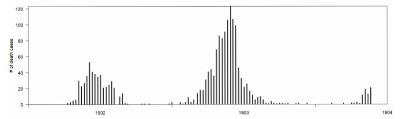
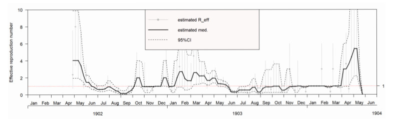
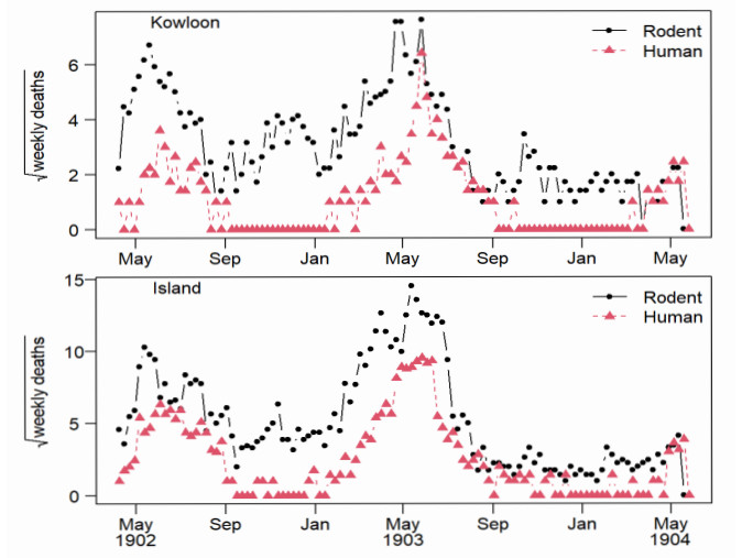
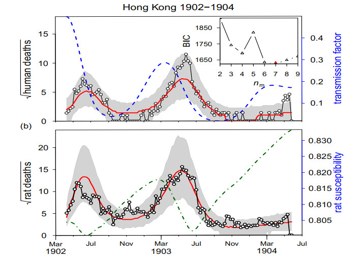
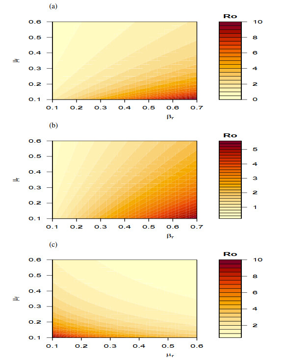
Identifying epidemic-driving factors through epidemiological modeling is a crucial public health strategy that has substantial policy implications for control and prevention initiatives. In this study, we employ dynamic modeling to investigate the transmission dynamics of pneumonic plague epidemics in Hong Kong from 1902 to 1904. Through the integration of human, flea, and rodent populations, we analyze the long-term changing trends and identify the epidemic-driving factors that influence pneumonic plague outbreaks. We examine the dynamics of the model and derive epidemic metrics, such as reproduction numbers, that are used to assess the effectiveness of intervention. By fitting our model to historical pneumonic plague data, we accurately capture the incidence curves observed during the epidemic periods, which reveals some crucial insights into the dynamics of pneumonic plague transmission by identifying the epidemic driving factors and quantities such as the lifespan of flea vectors, the rate of rodent spread, as well as demographic parameters. We emphasize that effective control measures must be prioritized for the elimination of fleas and rodent vectors to mitigate future plague outbreaks. These findings underscore the significance of proactive intervention strategies in managing infectious diseases and informing public health policies.
- plague,
- epidemiological modeling,
- reproduction number,
- epidemic
Citation: Salihu S. Musa, Shi Zhao, Winnie Mkandawire, Andrés Colubri, Daihai He. An epidemiological modeling investigation of the long-term changing dynamics of the plague epidemics in Hong Kong[J]. Mathematical Biosciences and Engineering, 2024, 21(10): 7435-7453. doi: 10.3934/mbe.2024327

Related Papers:

Abstract

Identifying epidemic-driving factors through epidemiological modeling is a crucial public health strategy that has substantial policy implications for control and prevention initiatives. In this study, we employ dynamic modeling to investigate the transmission dynamics of pneumonic plague epidemics in Hong Kong from 1902 to 1904. Through the integration of human, flea, and rodent populations, we analyze the long-term changing trends and identify the epidemic-driving factors that influence pneumonic plague outbreaks. We examine the dynamics of the model and derive epidemic metrics, such as reproduction numbers, that are used to assess the effectiveness of intervention. By fitting our model to historical pneumonic plague data, we accurately capture the incidence curves observed during the epidemic periods, which reveals some crucial insights into the dynamics of pneumonic plague transmission by identifying the epidemic driving factors and quantities such as the lifespan of flea vectors, the rate of rodent spread, as well as demographic parameters. We emphasize that effective control measures must be prioritized for the elimination of fleas and rodent vectors to mitigate future plague outbreaks. These findings underscore the significance of proactive intervention strategies in managing infectious diseases and informing public health policies.

References

[1]	World Health Organization, Plague, Keyfacts, 2023. Available from: https://www.who.int/news-room/fact-sheets/detail/plague.
[2]	Centers for Disease Control and Prevention, Plague, 2023. Available from: https://www.cdc.gov/plague/index.html.
[3]	Statista, Number of deaths due to plague in Hong Kong during the Third Plague Pandemic from 1894 to 1902, 2023. Available from: https://www.statista.com/statistics/1115206/annual-plague-deaths-hong-kong-third-plague-pandemic/.
[4]	K. R. Dean, F. Krauer, L. Walløe, O. C. Lingjærde, B. Bramanti, N. Chr. Stenseth, et al., Human ectoparasites and the spread of plague in Europe during the Second Pandemic, Proc. Nat. Acad. Sci., 115 (2018), 1304–9. https://doi.org/10.1073/pnas.1715640115 doi: 10.1073/pnas.1715640115
[5]	M. J. Keeling, C. A. Gilligan, Bubonic plague: a metapopulation model of a zoonosis, Proc. R. Soc. Lond. B, 267 (2000), 2219–2230. https://doi.org/10.1098/rspb.2000.1272. doi: 10.1098/rspb.2000.1272
[6]	V. K. Nguyen, C. Parra-Rojas, E. A. Hernandez-Vargas, The 2017 plague outbreak in Madagascar: Data descriptions and epidemic modelling, Epidemics, 25 (2018), 20–25. https://doi.org/10.1016/j.epidem.2018.05.001 doi: 10.1016/j.epidem.2018.05.001
[7]	World Health Organization, Plague manual: epidemiology, distribution, surveillance, and control, 1999. Available from: https://www.who.int/publications/i/item/WHO-CDS-CSR-EDC-99.2.
[8]	R. Yang, S. Atkinson, Z. Chen, Y. Cui, Z. Du, Y. Han, et al., Yersinia pestis and Plague: Some knowns and unknowns, Zoonoses (Burlington), 3 (2023), 5. https://doi.org/10.15212/zoonoses-2022-0040 doi: 10.15212/zoonoses-2022-0040
[9]	Center for Health Protection, Hong Kong, Scientific committee on vector-borne diseases, situation of plague and prevention strategies, 2024. Available from: https://www.chp.gov.hk/files/pdf/diseases-situation_of_plague_and_prevention_strategie_r.pdf.
[10]	E. H. Hankin, On the epidemiology of plague, Epidem. Infect., 5 (1905), 48–83.
[11]	R. Barbieri, M. Signoli, D. Chevé, C. Costedoat, S. Tzortzis, G. Aboudharam, et al., Yersinia pestis: the natural history of plague, Clin. Microbiol. Rev., 34 (2020), 10–128. https://doi.org/10.1128/CMR.00044-19 doi: 10.1128/CMR.00044-19
[12]	R. J. Eisen, S. W. Bearden, A. P. Wilder, J. A. Montenieri, M. F. Antolin, K. L. Gage, Early-phase transmission of Yersinia pestis by unblocked fleas as a mechanism explaining rapidly spreading plague epizootics, PNAS, 103 (2006), 15380–15385. https://doi.org/10.1073pnas.0606831103/
[13]	J. M. Girard, D. M. Wagner, A. J. Vogler, C. Keys, C. J. Allender, L. C. Drickamer, et al., Differential plague-transmission dynamics determine Yersinia pestis population genetic structure on local, regional, and global scales, PNAS, 101 (2004), 8408–8413. https://doi.org/10.1073/pnas.0401561101 doi: 10.1073/pnas.0401561101
[14]	K. A. Boegler, C. B. Graham, T. L. Johnson, J. A. Montenieri, R. J. Eisen, Infection prevalence, bacterial loads, and transmission efficiency in Oropsylla montana (Siphonaptera: Ceratophyllidae) one day after exposure to varying concentrations of Yersinia pestis in blood, J. Med. Entomol., 53 (2016), 674–680. https://doi.org/10.1093/jme/tjw004 doi: 10.1093/jme/tjw004
[15]	X. Didelot, L. K. Whittles, I. Hall, Model-based analysis of an outbreak of bubonic plague in Cairo in 1801, J. R. Soc. Interface, 14 (2017), 20170160. https://doi.org/10.1098/rsif.2017.0160 doi: 10.1098/rsif.2017.0160
[16]	S. Zhao, Z. Yang, S. S. Musa, J. Ran, M. K. C. Chong, M. Javanbakht, et al., Attach importance of the bootstrap t test against Student's t test in clinical epidemiology: a demonstrative comparison using COVID-19 as an example, Epidemiol. Infect., 149 (2021), e107. https://doi.org/10.1017/S0950268821001047 doi: 10.1017/S0950268821001047
[17]	K. R. Dean, F. Krauer, B. V. Schmid, Epidemiology of a bubonic plague outbreak in Glasgow, Scotland in 1900, R. Soc. open Sci., 6 (2019), 181695. https://doi.org/10.1098/rsos.181695 doi: 10.1098/rsos.181695
[18]	W. Hunter, A Research into Epidemic and Epizootic Plague, Hong Kong: Noronha & Co., 1904.
[19]	H. Nishiura, M. Kakehashi, Real time estimation of reproduction numbers based on case notifications-Effective reproduction number of primary pneumonic plague, Trop. Med. Health, 33 (2005), 127–32. https://doi.org/10.2149/tmh.33.127 doi: 10.2149/tmh.33.127
[20]	H. Nishiura, Backcalculation of the disease-age specific frequency of secondary transmission of primary pneumonic plague, preprint, arXiv: 0810.1606.
[21]	S. S. Musa, S. Zhao, D. Gao, Q. Lin, G. Chowell, D. He, Mechanistic modelling of the large-scale Lassa fever epidemics in Nigeria from 2016 to 2019, J. Theoret. Biol., 493 (2020), 110209. https://doi.org/10.1016/j.jtbi.2020.110209 doi: 10.1016/j.jtbi.2020.110209
[22]	S. Zhao, L. Stone, D. Gao, D. He, Modelling the large-scale yellow fever outbreak in Luanda, Angola, and the impact of vaccination, PLoS Neglet. Trop. Dis., 12 (2018), e0006158. https://doi.org/10.1371/journal.pntd.0006158 doi: 10.1371/journal.pntd.0006158
[23]	C. Breto, D. He, E. L. Ionides, A. A. King, Time series analysis via mechanistic models, Ann. Appl. Stat., 3 (2009), 319–348. http://dx.doi.org/10.1214/08-AOAS201 doi: 10.1214/08-AOAS201
[24]	S. S. Musa, A. Tariq, L. Yuan, W. Haozhen, D. He, Infection fatality rate and infection attack rate of COVID-19 in South American countries, Infect. Dis. Poverty, 11 (2022). https://doi.org/10.1186/s40249-022-00961-5
[25]	S. S. Musa, X. Wang, S. Zhao, S. Li, N. Hussaini, W. Wang, et al., The heterogeneous severity of COVID-19 in African countries: a modeling approach, Bull. Math. Biol., 84 (2022), 32. https://doi.org/10.1007/s11538-022-00992-x doi: 10.1007/s11538-022-00992-x
[26]	Q. Lin, Z. Lin, A. P. Y. Chiu, D. He, Seasonality of influenza A(H7N9) virus in China-fitting simple epidemic models to human cases, PLoS One, 11 (2016), e0151333. https://doi.org/10.1371/journal.pone.0151333 doi: 10.1371/journal.pone.0151333
[27]	D. He, E. L. Ionides, A. A. King, Plug-and-play inference for disease dynamics: measles in large and small populations as a case study, J. R. Soc. Interf., 7 (2010), 271–283. https://doi.org/10.1098/rsif.2009.0151 doi: 10.1098/rsif.2009.0151
[28]	D. He, S. Zhao, Q. Lin, S. S. Musa, L. Stone, New estimates of the Zika virus epidemic attack rate in Northeastern Brazil from 2015 to 2016: A modelling analysis based on Guillain-Barré Syndrome (GBS) surveillance data, PLoS Negl. Trop. Dis., 14 (2020), e0007502. https://doi.org/10.1371/journal.pntd.0007502 doi: 10.1371/journal.pntd.0007502
[29]	S. S. Musa, A. Tariq, L. Yuan, W. Haozhen, D. He, Infection fatality rate and infection attack rate of COVID-19 in South American countries, Infect. Dis. Poverty, 11 (2022), 42–52. https://doi.org/10.1186/s40249-022-00961-5 doi: 10.1186/s40249-022-00961-5
[30]	Partially Observed Markov Process (POMP), The website of $\texttt{R}$ package POMP: statistical inference for partially-observed Markov processes, 2018. Available from: https://kingaa.github.io/pomp/.
[31]	A. Camacho, S. Ballesteros, A. L. Graham, F. Carrat, O. Ratmann, B. Cazelles, Explaining rapid reinfections in multiple-wave influenza outbreaks: Tristan da Cunha 1971 epidemic as a case study, Proc. Biol. Sci., 278 (2011), 3635–3643. https://doi.org/10.1098/rspb.2011.0300 doi: 10.1098/rspb.2011.0300
[32]	World Bank, World Bank data, Population, total (years) - Hong Kong SARS, China, 2020. Available from: https://data.worldbank.org/country/hong-kong-sar-china?view = chart.
[33]	World Bank, World Bank data, Life expectancy at birth, total (years) - Hong Kong SAR, China, 2021. Available from: https://data.worldbank.org/indicator/SP.DYN.LE00.IN?locations = HK.
[34]	D. Gao, Y. Lou, D. He, T. C. Porco, Y. Kuang, G. Chowell, et al., Prevention and control of Zika as a mosquito-borne and sexually transmitted disease: a mathematical modeling analysis, Sci. Rep., 6 (2016), 28070. https://doi.org/10.1038/srep28070 doi: 10.1038/srep28070
[35]	D. He, S. Zhao, Q. Lin, S. S. Musa, L. Stone, New estimates of the Zika virus epidemic attack rate in Northeastern Brazil from 2015 to 2016: A modelling analysis based on Guillain-Barré Syndrome (GBS) surveillance data, PLoS Negl. Trop. Dis., 14 (2020), e0007502. https://doi.org/10.1371/journal.pntd.0007502 doi: 10.1371/journal.pntd.0007502
[36]	F. Krauer, H. Viljugrein, K. R. Dean, The influence of temperature on the seasonality of historical plague outbreaks, Proc. R. Soci. B., 288 (2021), 20202725. https://doi.org/10.1098/rspb.2020.2725 doi: 10.1098/rspb.2020.2725
[37]	J. Klunk, T. P. Vilgalys, C. E. Demeure, X. Cheng, M. Shiratori, J. Madej, et al., Evolution of immune genes is associated with the Black Death, Nature, 611 (2022), 312–319. https://doi.org/10.1038/s41586-022-05349-x doi: 10.1038/s41586-022-05349-x
[38]	P. van den Driessche, J. Watmough, Reproduction numbers and sub-threshold endemic equilibria for compartmental models of disease transmission, Math. Biosci., 180 (2002), 29–48, https://doi.org/10.1016/S0025-5564(02)00108-6 doi: 10.1016/S0025-5564(02)00108-6
[39]	O. Diekmann, J. Heesterbeek, J. Metz, On the definition and the computation of the basic reproduction ratio $R_0$ in models for infectious diseases in heterogeneous populations, J. Math. Biol., 28 (1990), 365–382. https://doi.org/10.1007/BF00178324 doi: 10.1007/BF00178324
[40]	P. van den Driessche, Reproduction numbers of infectious disease models, Infect. Dis. Model., 2 (2017), 288–303. https://doi.org/10.1016/j.idm.2017.06.002 doi: 10.1016/j.idm.2017.06.002
[41]	S. S. Musa, S. Zhao, D. He, C. Liu, The long-term periodic patterns of global rabies epidemics among animals: A modeling analysis, Int. J. Bifur. Chaos, 30 (2020), 2050047. https://doi.org/10.1142/S0218127420500479 doi: 10.1142/S0218127420500479
[42]	S. S. Musa, S. Zhao, N. Hussaini, S. Usaini, D. He, Dynamics analysis of typhoid fever with public health education programs and final epidemic size relation, Results Appl. Math., 10 (2021), 100153. https://doi.org/10.1016/j.rinam.2021.100153 doi: 10.1016/j.rinam.2021.100153
[43]	S. S. Musa, S. Zhao, N. Hussaini, A. G. Habib, D. He, Mathematical modeling and analysis of meningococcal meningitis transmission dynamics, Int. J. Biomath., 13 (2020), 2050006. https://doi.org/10.1142/S1793524520500060 doi: 10.1142/S1793524520500060

Reader Comments

Your name:*

Email:*
© 2024 the Author(s), licensee AIMS Press. This is an open access article distributed under the terms of the Creative Commons Attribution License (http://creativecommons.org/licenses/by/4.0)