


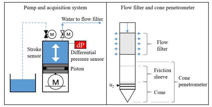
Figure 1.
Flow cone equipment including control system, flow filter and cone penetrometer.
Citation: Aleksander S. Gundersen, Pasquale Carotenuto, Tom Lunne, Axel Walta, Per M. Sparrevik. Field verification tests of the newly developed flow cone tool—In-situ measurements of hydraulic soil properties[J]. AIMS Geosciences, 2019, 5(4): 784-803. doi: 10.3934/geosci.2019.4.784
| [1] | Øyvind Blaker, Roselyn Carroll, Priscilla Paniagua, Don J. DeGroot, Jean-Sebastien L'Heureux . Halden research site: geotechnical characterization of a post glacial silt. AIMS Geosciences, 2019, 5(2): 184-234. doi: 10.3934/geosci.2019.2.184 |
| [2] | Aleksander S. Gundersen, Ragnhild C. Hansen, Tom Lunne, Jean-Sebastien L’Heureux, Stein O. Strandvik . Characterization and engineering properties of the NGTS Onsøy soft clay site. AIMS Geosciences, 2019, 5(3): 665-703. doi: 10.3934/geosci.2019.3.665 |
| [3] | Laura Tonni, Guido Gottard . Assessing compressibility characteristics of silty soils from CPTU: lessons learnt from the Treporti Test Site, Venetian Lagoon (Italy). AIMS Geosciences, 2019, 5(2): 117-144. doi: 10.3934/geosci.2019.2.117 |
| [4] | Efthymios Panagiotis, Alena Zhelezova, Irene Rocchi . Analysis of CPTu data from the North Sea region to estimate the frequency of inaccurate pore pressure measurements. AIMS Geosciences, 2025, 11(2): 517-527. doi: 10.3934/geosci.2025021 |
| [5] | Annika Bihs, Mike Long, Steinar Nordal . Geotechnical characterization of Halsen-Stjørdal silt, Norway. AIMS Geosciences, 2020, 6(3): 355-377. doi: 10.3934/geosci.2020020 |
| [6] | Annika Bihs, Mike Long, Steinar Nordal, Priscilla Paniagua . Consolidation parameters in silts from varied rate CPTU tests. AIMS Geosciences, 2021, 7(4): 637-668. doi: 10.3934/geosci.2021039 |
| [7] | Islam Marzouk, Andreas Erdian Wijaya, Helmut F Schweiger, Franz Tschuchnigg . An automated system for determining soil parameters from in situ tests: Application to a sand site. AIMS Geosciences, 2025, 11(2): 489-516. doi: 10.3934/geosci.2025020 |
| [8] | David Igoe, Kenneth Gavin . Characterization of the Blessington sand geotechnical test site. AIMS Geosciences, 2019, 5(2): 145-162. doi: 10.3934/geosci.2019.2.145 |
| [9] | Andrew C. Stolte, Brady R. Cox . Feasibility of in-situ evaluation of soil void ratio in clean sands using high resolution measurements of Vp and Vs from DPCH testing. AIMS Geosciences, 2019, 5(4): 723-749. doi: 10.3934/geosci.2019.4.723 |
| [10] | Elvis Ishimwe, Richard A. Coffman, Kyle M. Rollins . Predicting blast-induced liquefaction within the New Madrid Seismic Zone. AIMS Geosciences, 2020, 6(1): 71-91. doi: 10.3934/geosci.2020006 |
In geotechnical engineering, steady state and transient flow analyses are based on Darcy's law for laminar flow which relates discharge velocity, v, to hydraulic gradient, i, by the coefficient of permeability, k [1]. The coefficient of permeability represents the ease with which a fluid can flow through pore spaces, and is denoted hydraulic conductivity if the fluid is water [2]. In design, more attention is often directed towards the analysis method rather than the input of hydraulic conductivity itself, which may lead to unreliable results. No other property of importance is likely to exhibit an equivalently large range of values. From coarse grained to fine grained soils, the hydraulic conductivity may change by up to 10 orders of magnitude [3]. The permeability of granular soils depends mainly on the cross-sectional area of the pore channels, which is strongly influenced by the properties of the smallest grain sizes [4,5].
For in-situ prediction of rock permeability and permeability of dam materials, Lugeon [6] introduced a water pumping test in 1933, referred to as Packer or Lugeon test. For soil sediments, the framework proposed by Hvorslev [7] can be used to estimate hydraulic conductivities from falling head tests. The cone penetration test (CPTU) is relatively quick and there is a substantial amount of results available in literature. However, it is challenging to provide accurate determination of hydraulic properties from these results. More recent tools combine CPTU with flow filters facilitating constant flow rate into surrounding soil while cone penetration takes place [8].
NGI has developed a prototype tool for in-situ measurements of hydraulic properties of sands and silts, the flow cone. The tool combines the widely used cone penetrometer with a bronze filter located behind the cone penetrometer. The filter is connected to a pump and data acquisition system. Quinteros et al. (2019) [9,10] describes the ground conditions at the NGTS sand site (20 km south of Trondheim) at which the flow cone was tested. The purpose of the tool is to estimate the hydraulic soil properties quickly, reliably and easily.
This paper describes the in-situ testing and present the measured and interpreted results. The soil response types and the aspects of hydraulic conductivity from flow cone are discussed. The flow cone results are qualitatively compared to results from cone penetration tests, in-situ falling head tests, grain size distributions and constant head tests from laboratory. Recommendations for further testing are provided and potential application in engineering practice is outlined.
The flow cone is a standard cone penetrometer paired with a custom hydraulic module as illustrated in Figure 1. The hydraulic module consists of a clog-resistant bronze filter located 82 cm behind the cone and a control system at ground surface. The cylindrical filter is 11.95 cm long and has a radius of 1.84 cm. The control system handles data acquisition and provides flow rate control by means of a linear step motor driving a piston (see Figure 1). The ambient pressure, system pressure and flow rate are recorded by the data acquisition system. During testing, the two pressure sensors are located 1.4 m above ground level (marked by "dP" in Figure 1). The hydraulic tubing has an inner diameter of 6.5 mm and connects the bronze filter to the control system. The CPTU logs the standard parameters [11] and communicates these real-time to the surface acoustically.
For explanatory reasons, the flow cone testing is divided into cone penetration phase and stationary phase. The cone penetration phase is a standard cone penetration test [11,12] combined with constant water flow applied through the flow filter into the surrounding soil (see blue arrows in Figure 1). The purpose of the water flow during cone penetration is to keep the system fully saturated and prevent filter clogging. This study suggests that the penetration phase results may be calibrated to the hydraulic conductivity from stationary phase to establish a hydraulic conductivity profile (see Section 4.2). The penetration phase measurements may also be used to empirically estimate the hydraulic conductivity profile [8]. Based on the penetration phase results, the operator determines whether the penetration should be paused for stationary phase testing. For stationary phase testing, the flow cone features the three test types in Figure 2 i.e. constant head tests, constant flow rate tests and falling head tests.
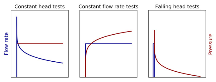
Table 1 presents the overview of measured parameters for the two different test phases. To obtain the pore pressure at flow filter location, the weight of the water column inside the tubes was added to the measured water pressure 1.4 m above ground level.
| Measured parameter | Test phase |
| Time, t | Both phases |
| Pore pressure at center of filter, uf, m | Both phases |
| Flow rate of water, Q | Both phases |
| Depth below ground level, z | Penetration phase |
| Cone resistance, qc | Penetration phase |
| Sleeve friction, fs | Penetration phase |
| Pore pressure measured behind cone, u2 | Penetration phase |
 DownLoad:
CSV
DownLoad:
CSV
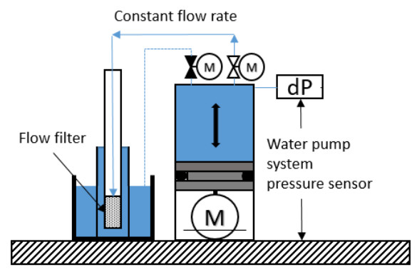
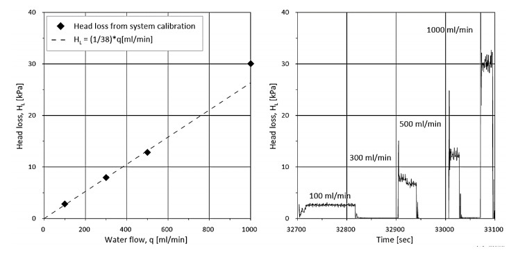
The resistance to water flow from the flow cone system itself was measured in the field. Figure 3 illustrates the setup for the system calibration. The flow filter was placed in a bucket topped with water, and different flow rates were specified to the pump and acquisition system. Figure 4 illustrates the measured pore pressure due to system friction (head loss, HL) with flow rate and time. Based on these results, Eq 1 was used to obtain the corrected pore pressure (uf, kPa) from the measured pore pressure (uf, m, kPa) and flow rate (Q, ml/min) for all tests at the NGTS sand site.
| (1) |
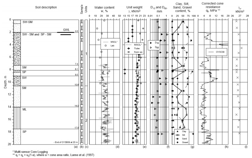
The flow cone testing was carried out at the NGTS sand site, which is a deltaic deposit about 20 km south of Trondheim, Norway. A significant number of in-situ tests have been carried out at the site including electrical piezometers, cone penetration testing (CPTU), falling head tests etc. The piezometers suggest that the elevation of the groundwater level (GWL) is on average 2 m below ground level. For borehole OYSB09, samples were retrieved using the Geonor 54 mm piston tube sampler, and constant head tests and grain size distribution tests were carried out by the NGI laboratory in Oslo.
The stratigraphy at the site comprises a gravelly sand layer within the top 6 m as illustrated by the borehole log in Figure 5. The dominating soil type below the gravelly sand layer is silty sand with varying contents of clay, silt and sand particles. The deposit is highly layered, and the soil stratigraphy may change from one location to another. The silt content varies from about 0% to 70% according to Figure 5.
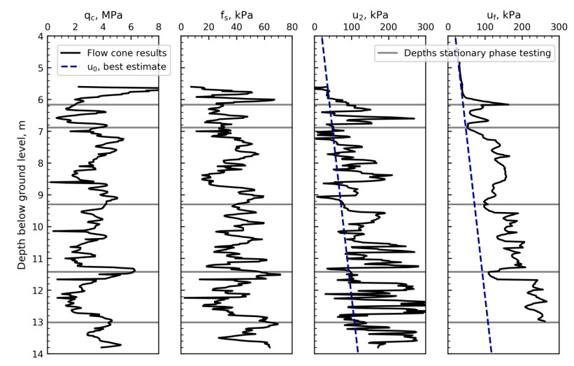
NGI carried out the flow cone tests on September 25, 2018. To prevent damages to the equipment, it was decided to predrill through the gravelly top layer. A constant flow rate of 50 ml/min was applied during the cone penetration, which was started from 5.6 m below ground level (bgl) and ended at 13.83 m bgl. The cone penetration was paused at the five depths considered most optimal for stationary phase testing based on the cone penetration results in Figure 6. Most emphasis was on the excess pore pressure, but also the sleeve friction and cone resistance were considered to optimize the stationary phase testing. Table 2 provides test depths (filter center), number of tests at each depth and specified flow rates for the stationary phase testing.
| Depth (m) | No. of tests | Flow rate (ml/min) |
| 6.16 | 5 | 100–300 |
| 6.88 | 5 | 100–300 |
| 9.30 | 3 | 12.3–24.6 |
| 11.42 | 8 | 16.4–400 |
| 13.01 | 4 | 8.2–100 |
DownLoad:
CSV
Figure 6 illustrates the measured cone resistance, qc, sleeve friction, fs, pore pressure behind cone, u2, and the pore pressure at flow filter center, uf, during the penetration phase. The figure includes best estimate in-situ pore pressure and the depths at which stationary phase tests were carried out. All parameters show variations with depth, which indicates a relatively layered soil profile. It is suggested that the local minimum pore pressures at flow filter location (e.g. 6.88 m bgl) correspond to layers with higher hydraulic conductivity (see Section 4.2). The local minimum pore pressures correspond well with three of the stationary phase test depths.
Figure 7 illustrates the pore pressure response at flow filter location 6.16 m bgl with time. Five tests with different flow rates were carried out at this depth as illustrated in the figure. The pore pressure for the three first tests quickly reaches a peak before rapidly decreasing down to a pressure plateau. Although the specified flow rates for the first two tests are identical to the last two tests, the resulting pore pressure for the last two tests are lower, which implies a change in soil structure has occurred.
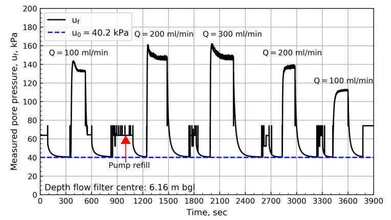
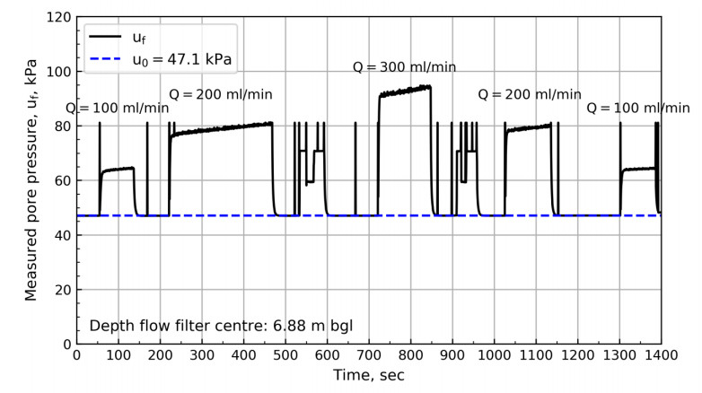
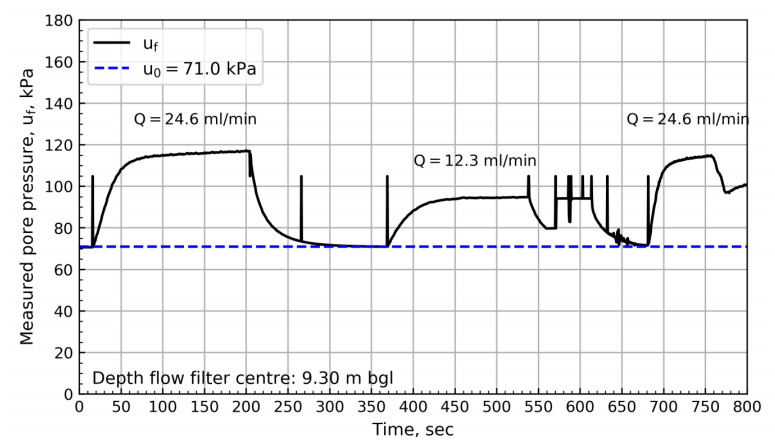
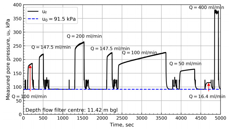
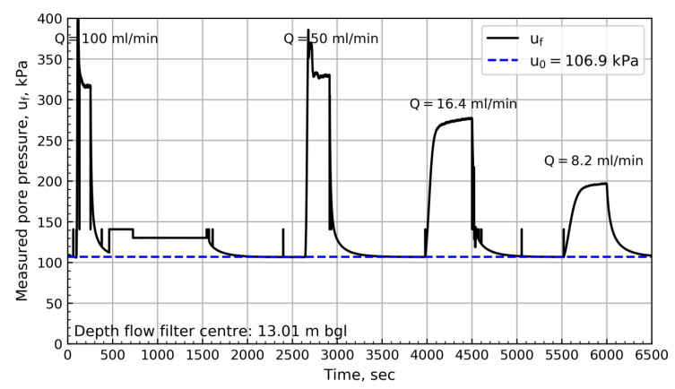
Figure 8 shows the results from 6.88 m bgl. These results show a swift change in pressure until reaching the pressure plateau. After reaching the plateau, a steady increase in pore pressure with time can be observed. The results from the NGTS sand site suggest that the slope of the plateau depends on the specified flow rate. Figures 9 to 11 show the pore pressure response for the remaining tests where different test sequences were investigated.
This section presents the interpretation of in-situ pore pressure and hydraulic conductivity from flow cone results. The hydraulic conductivity is compared to the results of various other tests at the NGTS sand site and the soil response types are discussed.
For the stationary phase testing, the excess pore pressure around the flow filter is allowed to dissipate before each flow rate is tested as illustrated in Figures 7 to 11. The pressure dissipation curves converge towards the static in-situ pore pressure, u0, which is required for further interpretation of the flow cone measurements. Figure 12 illustrates the in-situ pore pressures from all stationary phase testing with depth. In addition to the flow cone results, the measured results from five piezometers located less than 20 m away are included. The piezometer readings are from April 28, 2017 to May 31, 2018 and the pore pressures seem to vary with season and cycle of the moon [9]. The flow cone measurements are within the expected range of values based on the piezometer measurements. The pore pressure profile used in further interpretation of flow cone results is defined by Eq 2 and included in Figure 12 (z is depth below ground level).
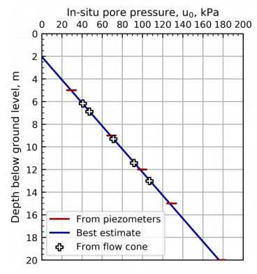
| (2) |
NGI [13] documents the flow cone feasibility study, in which constant head tests with the flow cone tool were simulated using finite elements (FE). The axisymmetric FE model comprised one soil layer with a linear elastic material behavior and the tool geometry as illustrated in Figure 13. The finite element mesh was refined in the vicinity of the flow filter. Figure 13b) illustrates the resulting contours of pressure head around the flow filter i.e. the pressure head distribution within the soil volume. For undisturbed soil and laminar flow, the study suggested that there exists a linear relationship between pressure head, H = uf – u0, and flow rate, Q. The hydraulic conductivities used as input to the finite element analyses were identical to the hydraulic conductivities derived from Eq 3 [14].
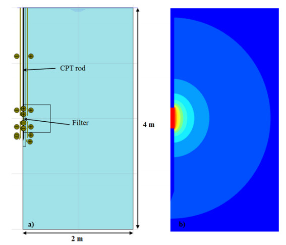
| (3) |
here, L and r are the filter length and radius respectively. Q is the rate of water flow in cubic meter per second and H is the pressure head in meters. For the testing at Øysand, the filter length was 11.95 cm and the filter radius was 1.84 cm, hence the constant C becomes 2.49 m−1.
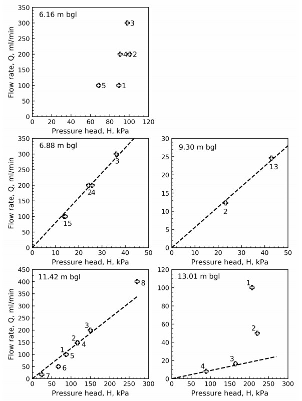
Figure 14 illustrates the pressure head taken from the start of each pressure plateau (see Figures 7 to 11) with flow rate. Data labels show the test sequence at each depth and dashed lines represent the proposed linear relationship between flow rate and pressure head at the different depths. No linear relationship was suggested for depth 6.16 m bgl where the testing may have been influenced by erosion and/or cracking. Figures 7 to 11 and Figure 14 suggest that soil disturbance due to water flow occurred for tests at depths 6.16 m bgl and 13.01 m bgl. The reason for this is that excessive flow rates relative to the soil types encountered were specified. Figure 15 illustrates the hydraulic conductivity derived from Eq 3 and the dashed lines in Figure 14.
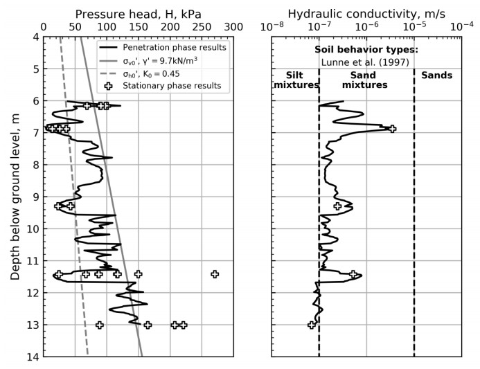
Laminar flow may not be expected for the cone penetration phase, hence the interpretation of hydraulic conductivity suggested by FE analyses may not be applicable. To be able to estimate the hydraulic conductivity profile, the hydraulic conductivity from penetration phase using Eq 3 was shifted by modifying the constant C (see Eq 3). The constant C was modified so that the hydraulic conductivity from penetration phase and stationary phase are aligned at the depths of stationary testing (see Figure 15). Figure 15 illustrates the pressure head and hydraulic conductivity from stationary phase (points) and penetration phase (continuous line) with depth. The in-situ vertical and horizontal effective stresses are included for comparison. The figure shows that the pressure head exceeds the in-situ horizontal and vertical effective stresses for some of the tests, e.g. at 6.2 m, 11.4 m and 13 m depth. Soil behavior types presented by Lunne et al. [12] are included in the hydraulic conductivity profile for comparison. The hydraulic conductivity plot suggests that the soil behavior is mainly sand mixtures or silty sand, and there are three layers with high permeability compared to other test depths.
Figure 16 illustrates the corrected cone resistance (qt), soil behavior type index (IC), and estimated hydraulic conductivity with depth for several tests at the NGTS sand site. Soil behavior type boundaries from Lunne et al. [12] have been included for comparison. The hydraulic conductivity was estimated from flow cone tests, in-situ falling head tests, grain size distribution and constant head tests in the laboratory.
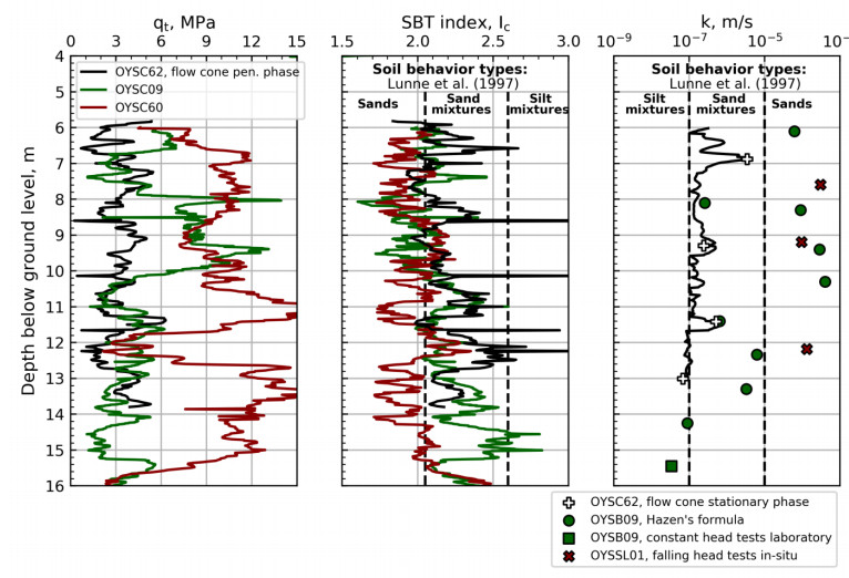
Four in-situ falling head tests have been carried out close to cone penetration test OYSC60, for which the time lag method [7] was used to interpret the hydraulic conductivity. The results of the cone penetration test (red continuous line) and falling head tests (red crosses, one test above depth range in the figure) are included in Figure 16. The cone resistance from OYSC60 is about twice the cone resistance from flow cone, suggesting different soil conditions. It is expected that the hydraulic conductivity is higher at this location based on the cone penetration results, and the hydraulic conductivities seem to support this.
A range of tests has been carried out on samples from borehole OYSB09 as illustrated in the borehole log in Figure 5. The borehole log illustrates the contents of clay, silt and sand, and the grain sizes corresponding to 10% (d10, mm) and 60% (d60, mm) of passed material. The hydraulic conductivities using Eq 4 [4], based on the 10 % grain size, are illustrated in Figure 16.
| (4) |
These results are in line with the flow cone results at depths 8.1 m, 11.4 m and 14.2 m (visual extrapolation) bgl. However, there are large differences in the rest of the profile, which may not be explained by the difference in soil type identified by the CPTU results. For depth ranges 6 m to 6.5 m and 8 m to 10 m, it is evident that the cone resistance from OYSC09 is higher than the flow cone. It should be noted that the hydraulic conductivity from Eq 4 ranges from 10−7 m/s to about 10−3 m/s, i.e. range of four orders of magnitude.
The hydraulic conductivity from one constant head test (15.45 m bgl) in the laboratory is included in Figure 16. The specimen was loaded to a best estimate of the in-situ stresses. This result is in line with the trend of the hydraulic conductivity profile from flow cone as seen in the figure.
The Packer, or Lugeon, test was originally introduced by Lugeon [6] and is widely used to estimate the permeability of dam materials and rocks. The principles of this test are similar to the principles of the flow cone test. There are generally five response types identified for Packer testing in rocks not considering impervious rocks [15,16,17]. In accordance with Houlsby [15], these types are; A—laminar flow, B—turbulent flow, C—dilation, D—erosion or cracking and E—void filling. The different response types are illustrated in Figure 17 in pressure head (P) versus flow rate (Q) plots. In line with this interpretation, it is believed that two main response types can be identified from the stationary flow cone results by comparing Figures 14 and 17.
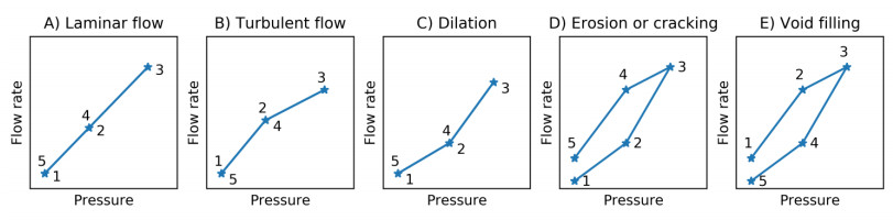
The test results at 6.16 m depth in Figure 14 suggest that erosion or cracking has occurred. This may also be indicated by the results in Figure 7, where the water pressure quickly reaches a maximum, followed by rapid pressure decrease towards a pressure plateau. This response type may also be observed from Figures 10 and 11, and is attributed to excessive hydraulic gradients resulting from specifying excessive flow rates for the soil types encountered.
Laminar flow is identified from Figure 14 at depths 6.88 m, 9.30 m and 11.42 m, where the results suggest a linear relationship between pressure head and flow rate.
For reliable estimation of hydraulic conductivity, a set of challenges and uncertainties were identified from the testing at Øysand. The challenges and potential mitigations are summarized in Table 3 and described in the following subsections.
| Challenge/Uncertainty | Mitigation/Further studies |
| Hydraulic fracture, erosion | Reduce flow rate, constant head test |
| Small difference between measured pore pressure and in-situ pore pressure | Increase flow rate |
| Laminar or turbulent flow | Review of pressure versus flow rate curve |
| Zone of influence, soil layering | FE analyses and model testing |
| Applicability of Eq 3 | FE analyses |
DownLoad:
CSV
The amount of soil disturbance during flow cone testing depends on the hydraulic gradient. Excessive gradients leads to erosion or redistribution of soil particles, potentially piping and/or hydraulic fracturing. A potential mitigation is to reduce the specified flow rate or carry out constant head testing. If the aim is to estimate hydraulic properties below a critical gradient, it is recommended to target pressure heads smaller than the in-situ vertical effective stress. Eq 3 can be used to estimate the pressure head before going to the field for the expected range of hydraulic conductivities.
The equation used for interpretation herein is ill-conditioned if the pressure head is small, which can be avoided by specifying the pressure head or by specifying higher water flow where appropriate. For the penetration phase at Øysand, a constant flow rate of 50 ml/min was specified. For testing in coarser material, it is recommended to increase the flow rate during penetration and the volume of the water container.
At Øysand, the number of tests at each depth ranged from three to eight. For the two shallowest depths, five tests with three flow rates were specified. The lowest flow rate was specified for the first and fifth tests and the intermediate flow rate was specified for the second and fourth tests. This test sequence was found to be beneficial for interpretation, providing information on the influence of previous testing on the results and assessment of flow type. This approach is similar to the Packer test procedure and laboratory testing of hydraulic conductivity.
Laboratory tests are often carried out on small soil samples and the results thus represent a small element within the total soil volume. The hydraulic conductivity from flow cone tests, and other in-situ permeability tests, may be influenced by the soil layering in-situ which may be a source of error when comparing with laboratory test results.
Hydraulic conductivity for a range of porosities can be determined from laboratory testing while the flow cone results are only valid for the in-situ porosity, which may be altered due to remolding of soil surrounding the cone. As described in Section 4.2, flow cone testing in a single soil layer was modelled using finite elements as part of the flow cone feasibility study [13]. The results showed that a remolded zone with different hydraulic properties lead to erroneous estimates on hydraulic conductivity using Eq 3. The feasibility study showed that increasing the filter length made the prediction of hydraulic conductivity using Eq 3 more independent of the remolded zone. It is recommended to study the effect of soil properties and soil layering using finite element analyses. Back calculation of the results from Øysand could yield a link between flow cone results and coefficient of consolidation.
With current test setup, the flow rate and water pressures are measured with high accuracy above ground level. The pore pressures are therefore corrected for vertical distance to the flow filter, and internal friction. For further testing it is recommended to measure the pore pressure and water flow at the location of the flow filter to reduce potential uncertainties related to the system itself. Uncertainties may be erroneous calibration, system changes during testing and nonlinear flow resistance from system.
Depending on the location within the NGTS sand site, some variations in soil conditions are evident. Cone penetration testing close to the falling head test location suggests different layering compared to the flow cone test location. On that note, no benchmark test exists for the flow cone results. If further hydraulic testing at Øysand is to be considered, it is recommended to carry out a benchmark test nearby the flow cone test location. Sampling and grain size tests from the vicinity of flow cone test location is also beneficial for benchmarking.
In-situ methods offer quick and reliable information about soil conditions, however it may be difficult to distinguish different types of sands and silts based solely on these results. The grain size distribution on the other hand is widely used to define and differentiate types of sands and silts. The significant influence of the smallest soil particles on the hydraulic conductivity suggests that flow cone may improve the reliability of in-situ soil characterization.
There are many design cases that involve seepage analyses such as design of excavation pits and retaining wall, earth fill dams, tailings dams etc. For excavations it is important to reliably estimate the amount of water flowing into the excavation and whether the hydraulic gradients may cause hydraulic fracturing. This study suggests that predictions can be improved if good quality flow cone results are available.
The behavior of suction bucket jackets during installation in silts and sands is difficult to estimate. One key to understanding the behavior is to have reliable information on the flow pattern and hydraulic properties of the soil. A potential advantage of the flow cone over laboratory testing (in addition to costs) is that a larger part of the soil profile may influence the results, and the results may therefore be more representative.
NGI has developed an in-situ prototype tool for estimation of hydraulic properties of sands and silts, the flow cone. The tool combines the widely used cone penetration test and a custom-made hydraulic module facilitating constant flow rate tests during cone penetration, and three types of hydraulic testing during stand-still (stationary phase testing). Pore pressures, water flow and time, in addition to standard CPTU parameters, are measured. Constant head tests with the tool have been simulated using finite elements. Based on finite element analyses results, an equation to estimate the hydraulic conductivity from stationary phase results has been suggested. The expected range of hydraulic conductivity for which the flow cone tool is applicable is from 10−8 m/s to 10−3 m/s and it is believed that the tool has potential as screening tool with site characterization purposes. The tool can also potentially provide important input parameters to seepage analyses and direct application for excavations, dams and suction bucket installation in sands and silts.
The tool was tested in the field at the NGTS sand site where the dominating soil type is silty sand. Stationary phase testing was carried out in one location at five different depths. The in-situ static pore pressure was determined from the flow cone excess pore pressure dissipation curves. These pore pressures are within the expected range of values based on measurements from electric piezometers permanently installed at the site.
The hydraulic conductivity was estimated from the equation suggested by finite element results and the proposed linear relationships between pressure head and flow rate for each depth. The hydraulic conductivity profile compares well with some of the results based on grain size distribution, in-situ falling head tests, and laboratory constant head tests. A silty sand soil type is suggested by comparing the hydraulic conductivity profile with soil behavior type boundaries available in literature. The hydraulic conductivity exhibits a variation of about 4 orders of magnitude (all test types and based on grain size alone) which is mainly attributed to the highly layered soil profile. In general, the flow cone results suggest a decreasing hydraulic conductivity with depth.
For the testing at Øysand, large hydraulic gradients may have caused soil disturbance potentially resulting in unreliable results. With the aim of reliable estimation of hydraulic conductivity, it is recommended to target pressure heads smaller than the in-situ vertical effective stress. Eq 3 can be used to estimate the pressure head before going to the field for the expected range of hydraulic conductivities.
This study was carried out within the SP9 project (NGI) funded by the Norwegian Research Council. The NGTS project contributed to the work presented herein. The authors would also like to thank colleagues at NGI for time spent on discussions, in addition to field operations department at NGI and everyone involved in the project.
All authors declare no conflicts of interest in this paper.
| [1] | Darcy H (1856) Les fontaines publiques de la ville de Dijon: exposition et application. Paris: Victor Dalmont. |
| [2] | Terzaghi K, Peck RB, Mesri G (1996) Soil mechanics in engineering practice. John Wiley & Sons. |
| [3] | Mitchell JK, Soga K (2005) Fundamentals of soil behavior. Third Edition, John Wiley & Sons New York. |
| [4] | Hazen A (1892) Physical properties of sands and gravels with reference to use in filtration. Report to Massachusetts State Board of Health, 539. |
| [5] | Kenney TC, Lau D, Ofoegbu GI (1984) Permeability of compacted granular materials. CanGeotech J 21: 726-729. |
| [6] | Lugeon M (1933) Barrages et Geologie. Dunod, Paris. |
| [7] | Hvorslev MJ (1951) Time lag and soil permeability in ground-water observations. |
| [8] | McCall W (2010) Tech guide for calculation of estimated hydraulic conductivity (Est. K) Log from HPT Data. Geoprobe System. |
| [9] |
Quinteros S, Gundersen AS, L'Heureux JS, et al. (2019) Øysand research site: Geotechnical characterisaiton of deltaic sandy-silty soils. AIMS Geosci 5: 750-783. doi: 10.3934/geosci.2019.4.750

|
| [10] | Gundersen AS, Quinteros S, L'Heureux JS, et al. (2018) Soil classification of NGTS sand site (Øysand, Norway) based on CPTU, DMT and laboratory results. Cone Penetration Testing IV: Proceedings of the 4th International Symposium on Cone Penetration Testing (CPT 2018), June 21-22, 2018, Delft, The Netherlands, 323. |
| [11] | ISO (2012) Geotechnical investigation and testing-Field testing. Part 1: Electrical cone and piezocone penetration test (ISO 22476-1). Geneva, Switzerland: International Organization for Standardization. |
| [12] | Lunne T, Powell JJ, Robertson PK (1997) Cone penetration testing in geotechnical practice. CRC Press. |
| [13] | NGI (2018) SP9-NGI Foundations-WP1-Technical Not-Summary 2016. Oslo: NGI. |
| [14] | BSI (1999) Code of practice for site investigations (BS 5930). London, United Kingdom: British Standard Institute. |
| [15] | Houlsby A (1976) Routine interpretation of the Lugeon water-test. Q J Eng Geol Hydrogeol 9: 303-313. |
| [16] | Kutzner C (1985) Considerations on rock permeability and grouting criteria. Proc the 15th Congress on Large Dams, 315-328. |
| [17] | Ewert FK (1994) Evaluation and interpretation of water pressure tests. Grouting in the ground: Proceedings of the conference organized by the Institution of Civil Engineers and held in London on 25-26 November 1992, Thomas Telford Publishing, 141-162. |
| 1. | Jean-Sebastien L’Heureux, Tom Lunne, Characterization and Engineering properties of Natural Soils used for Geotesting, 2020, 6, 2471-2132, 35, 10.3934/geosci.2020004 |
Aleksander S. Gundersen, Pasquale Carotenuto, Tom Lunne, Axel Walta, Per M. Sparrevik. Field verification tests of the newly developed flow cone tool—In-situ measurements of hydraulic soil properties[J]. AIMS Geosciences, 2019, 5(4): 784-803. doi: 10.3934/geosci.2019.4.784

| Measured parameter | Test phase |
| Time, t | Both phases |
| Pore pressure at center of filter, uf, m | Both phases |
| Flow rate of water, Q | Both phases |
| Depth below ground level, z | Penetration phase |
| Cone resistance, qc | Penetration phase |
| Sleeve friction, fs | Penetration phase |
| Pore pressure measured behind cone, u2 | Penetration phase |
DownLoad:
CSV
| Depth (m) | No. of tests | Flow rate (ml/min) |
| 6.16 | 5 | 100–300 |
| 6.88 | 5 | 100–300 |
| 9.30 | 3 | 12.3–24.6 |
| 11.42 | 8 | 16.4–400 |
| 13.01 | 4 | 8.2–100 |
DownLoad:
CSV
| Challenge/Uncertainty | Mitigation/Further studies |
| Hydraulic fracture, erosion | Reduce flow rate, constant head test |
| Small difference between measured pore pressure and in-situ pore pressure | Increase flow rate |
| Laminar or turbulent flow | Review of pressure versus flow rate curve |
| Zone of influence, soil layering | FE analyses and model testing |
| Applicability of Eq 3 | FE analyses |
DownLoad:
CSV
| Measured parameter | Test phase |
| Time, t | Both phases |
| Pore pressure at center of filter, uf, m | Both phases |
| Flow rate of water, Q | Both phases |
| Depth below ground level, z | Penetration phase |
| Cone resistance, qc | Penetration phase |
| Sleeve friction, fs | Penetration phase |
| Pore pressure measured behind cone, u2 | Penetration phase |
| Depth (m) | No. of tests | Flow rate (ml/min) |
| 6.16 | 5 | 100–300 |
| 6.88 | 5 | 100–300 |
| 9.30 | 3 | 12.3–24.6 |
| 11.42 | 8 | 16.4–400 |
| 13.01 | 4 | 8.2–100 |
| Challenge/Uncertainty | Mitigation/Further studies |
| Hydraulic fracture, erosion | Reduce flow rate, constant head test |
| Small difference between measured pore pressure and in-situ pore pressure | Increase flow rate |
| Laminar or turbulent flow | Review of pressure versus flow rate curve |
| Zone of influence, soil layering | FE analyses and model testing |
| Applicability of Eq 3 | FE analyses |

