Citation: Richard C Petersen. Free-radicals and advanced chemistries involved in cell membrane organization influence oxygen diffusion and pathology treatment[J]. AIMS Biophysics, 2017, 4(2): 240-283. doi: 10.3934/biophy.2017.2.240
[1] | Lazarus Kalvein Beay, Agus Suryanto, Isnani Darti, Trisilowati . Hopf bifurcation and stability analysis of the Rosenzweig-MacArthur predator-prey model with stage-structure in prey. Mathematical Biosciences and Engineering, 2020, 17(4): 4080-4097. doi: 10.3934/mbe.2020226 |
[2] | Kwangjoong Kim, Wonhyung Choi . Local dynamics and coexistence of predator–prey model with directional dispersal of predator. Mathematical Biosciences and Engineering, 2020, 17(6): 6737-6755. doi: 10.3934/mbe.2020351 |
[3] | Xue Xu, Yibo Wang, Yuwen Wang . Local bifurcation of a Ronsenzwing-MacArthur predator prey model with two prey-taxis. Mathematical Biosciences and Engineering, 2019, 16(4): 1786-1797. doi: 10.3934/mbe.2019086 |
[4] | William Wolesensky, J. David Logan . An individual, stochastic model of growth incorporating state-dependent risk and random foraging and climate. Mathematical Biosciences and Engineering, 2007, 4(1): 67-84. doi: 10.3934/mbe.2007.4.67 |
[5] | P. Auger, N. H. Du, N. T. Hieu . Evolution of Lotka-Volterra predator-prey systems under telegraph noise. Mathematical Biosciences and Engineering, 2009, 6(4): 683-700. doi: 10.3934/mbe.2009.6.683 |
[6] | Aniello Buonocore, Luigia Caputo, Enrica Pirozzi, Amelia G. Nobile . A non-autonomous stochastic predator-prey model. Mathematical Biosciences and Engineering, 2014, 11(2): 167-188. doi: 10.3934/mbe.2014.11.167 |
[7] | Yun Kang, Sourav Kumar Sasmal, Amiya Ranjan Bhowmick, Joydev Chattopadhyay . Dynamics of a predator-prey system with prey subject to Allee effects and disease. Mathematical Biosciences and Engineering, 2014, 11(4): 877-918. doi: 10.3934/mbe.2014.11.877 |
[8] | Nazanin Zaker, Christina A. Cobbold, Frithjof Lutscher . The effect of landscape fragmentation on Turing-pattern formation. Mathematical Biosciences and Engineering, 2022, 19(3): 2506-2537. doi: 10.3934/mbe.2022116 |
[9] | Jin Zhong, Yue Xia, Lijuan Chen, Fengde Chen . Dynamical analysis of a predator-prey system with fear-induced dispersal between patches. Mathematical Biosciences and Engineering, 2025, 22(5): 1159-1184. doi: 10.3934/mbe.2025042 |
[10] | Maoxiang Wang, Fenglan Hu, Meng Xu, Zhipeng Qiu . Keep, break and breakout in food chains with two and three species. Mathematical Biosciences and Engineering, 2021, 18(1): 817-836. doi: 10.3934/mbe.2021043 |
Spatial heterogeneity, dispersal patterns, and biotic interactions influence the distribution of species within a landscape [4, 47, 60, 68, 70]. Spatial self-organization results from local interactions between organisms and the environment, and emerges at patch-scales [61, 75]. For example, limited dispersal ability and its related dispersal patterns [57] is considered to be one of the key factors that promote the development of self-organized spatial patterns [1, 42, 71, 72].
In nature, especially for ecological communities of insects, dispersal of a predator is usually driven by its non-random foraging behavior which can often response to prey-contact stimuli [23], including spatial variation in prey density [40] and different types of signals arising directly from prey [76]. For instances, bloodsucking insects respond to the carbon dioxide output and the visual signals of a moving animal, which in tsetse flies (Glossina spp.) lead to the formation of a "following swarm" associated with herds of grazing ungulates [14, 34]. Most mosquitoes were attracted over a larger distance by the odor of the host [17, 18, 19]. The wood-wasp, Sirex noctilio, is attracted by the concentration of the scent [19, 53]. Social ants excite "pheromone trails" to encourage other individuals to visit the same food source [6]. Plant-feeding insects commonly detect food items by gustatory signals [65, 66, 66]. These non-random foraging behaviors driven by prey-mediated patch attractants, prey attractants themselves, and arrestant stimuli following the encounter of a prey, can lead to predation rates that are greater in regions where prey are more abundant (i.e., density-dependent predation), thus regulate population dynamics of both prey and predator.
Recent experimental work on population dynamics of immobile Aphids and Coccinellids by [44] show that the foraging movements of predator Coccinellids are combinations of passive diffusion, conspecific attraction, and retention on plants with high aphid numbers which is highly dependent on the strength of prey-predator interaction. Their study also demonstrates that predation by coccinellids was responsible for self-organization of aphid colonies. Many ecological systems exhibit similar foraging movements of predator. For example, Japanese beetles are attracted to feeding induced plant volatiles and congregate where feeding is taking place [52]. Motivated by these field studies, we propose a two-patch prey-predator model incorporating foraging movements of predator driven by the strength of prey-predator interaction, to explore how this non-random dispersal behavior of predator affect population dynamics of prey and predator.
Dispersal of predator plays an important role in regulating, stabilizing, or destabilizing population dynamics of both prey and predator. There are fair amount literature on mathematical models of prey-predator interactions in patchy environments. For example, see work of [47, 25, 3, 24, 26, 27, 64, 74, 20, 21, 62, 38, 39] and also see [41] for literature review. Many studies examine how the interactions between patches affect the synchronicity of the oscillations in each patch, e.g. see the work of [28, 35], and how interactions may stabilize or destabilize the dynamics. For instances, [37, 35] studied a model with two patches, each with the wellknown prey-predator Rosenzweig-McArthur dynamics, linked by the density independent dispersal (i.e., dispersal is driven by the difference of species' population densities in two patches). His study showed that this type of spatial predator-prey interactions might exhibit self-organization capable of producing stabilizing heterogeneities in prey distribution, and spatial populations can be regulated through the interplay of local dynamics and migration.
However, due to the intricacies that arise in density-dependent dispersal models, there are relatively limited work on models with non-random foraging behavior of predator or non-linear dispersal behavior [40] but see the two patch model with predator attraction to prey, e.g. [32], or predator attraction to conspecific, e.g. [58], or only predators migrate who are attracted to regions with concentrated food resources, see the work of [22, 8]. [40] proposed a non random foraging PDE model through a mechanistic approach to demonstrate that area-restricted search does yield predator aggregation, and explore the the consequences of area-restricted search for predator-prey dynamics. In addition, they provided many supporting ecological examples (e.g. Coccinellids, blackbirds, etc.) that abide by their theory. [32] studied a two-patch predator-prey Rosenzweig-MacArthur model with nonlinear density-dependent migration in the predator. The migration term of the predator is derived by extending the Holling time budget argument to migration. Their study showed that the extension of the Holling time budget argument to movement has essential effects on the dynamics. By extending the model of [32], [16] formulated a similar two patch prey-predator model with density-independent migration in prey and density-dependent migration in the predator. Their study shows that several foraging parameters such as handling time, dispersal rate can have important consequences in stability of prey-predator system. [10] investigated the population-dispersal dynamics for predator-prey interactions in a two patch environment with assumptions that both predators and their prey are mobile and their dispersal between patches is directed to the higher fitness patch. They proved that such dispersal, irrespectively of its speed, cannot destabilize a locally stable predator-prey population equilibrium that corresponds to no movement at all.
In this paper, we formulates a new version of Rosenzweig-MacArthur two patch prey predator model with mobility only in predator. Our model is distinct from others as we assume that the non-random foraging movements of predator is driven by the strength of prey-predator interactions, i.e., predators move towards patches with more concentrated prey and predator. Our model can apply to many insects systems such as Aphids and Coccinellids, Japanese beetles and their host plants, etc. For instance, the experimental work of [5] demonstrated that attraction to uninfested potato plants by Colorado potato beetle does not occur when the plants are small. However, when small plants are infested by conspecific larvae they become highly attractive to adult beetles. Thus predators beetles are are more attracted toward patches with high prey-predator interaction strength. The prey-predation attraction can also be observed in the field work of [44]. The main focus of our study of such prey-predator interactions in heterogeneous environments is to explore the following ecological questions:
1.How does our proposed nonlinear density-dependent dispersal of predator stabilize or destabilize the system?
2.How does dispersal of predator affect the extinction and persistence of prey and predator in both patches?
3.How may dispersal promote the coexistence of prey and predator when predator goes extinct in the single patch?
4.What are potential spatial patterns of prey and predator?
5.How are the effects of our proposed nonlinear density-dependent dispersal of predator on population dynamics different from the effects of the traditional density-independent dispersal?
The rest of the paper is organized as follows: In Section (2), we provide the detailed derivation of our two patch prey-predator model. In Section (3), we perform completed local and global dynamics of our model, and derive sufficient conditions that lead to the persistence and extinction of predator as well as permanence of the model. In Section (4), we perform bifurcation simulations to explore the dynamical patterns and compare the dynamics of our model to the traditional model [26, 27, 37, 35, 36]. In Section (5), we conclude our study and discuss the potential future study. The detailed proofs of our analytical results are provided in the last section.
Let
duidt=riui(1−uiki)−biuivi1+bihiuidvidt=cibiuivi1+bihiui−δivi | (1) |
where
We assume that the dispersal of predator from one patch to the other is driven by the strength of the prey-predator interaction in two patches which is termed as the attraction strength. More specifically, in the presence of dispersal, the dispersal rate of predators from Patch
bjujvj1+bjhjujρijvi−biuivi1+bihiuiρjivj | (2) |
where
du1dt=r1u1(1−u1k1)−b1u1v11+b1h1u1dv1dt=c1b1u1v11+b1h1u1−δ1v1+(b1u1v11+b1h1u1ρ21v2−b2u2v21+b2h2u2ρ12v1)du2dt=r2u2(1−u2k2)−b2u2v21+b2h2u2dv2dt=c2b2u2v21+b2h2u2−δ2v2+(b2u2v21+b2h2u2ρ12v1−b1u1v11+b1h1u1ρ21v2). | (3) |
We use the similar rescaling approach in [51] by letting
xi=bihiui,yi=bihicivi,Ki=bihiki,ai=cihi,di=ciδibihi, |
then we have
v1(b1u11+b1h1u1ρ21v2−b2u2v21+b2h2u2ρ12)=v1(b1x1b1h11+x1ρ21c2b2h2y2−b2x2b2h2c2b2h2y21+x2ρ12)=v1(ρ21a1a2c1b2x1y21+x1−ρ12a22c2b2x2y21+x2) |
and
v2(b2u21+b2h2u2ρ12v1−b1u1v11+b1h1u1ρ21)=v2(b2x2b2h21+x2ρ12c1b1h1y1−b1x1b1h1c1b1h1y11+x1ρ21)=v2(ρ12a1a2c2b1x2y11+x2−ρ21a21c1b1x1y11+x1) |
For mathematical convenience, we assume that
v1(ρ21a1a2c1b2x1y21+x1−ρ12a22c2b2x2y21+x2)=v1y2ρa2b2(a1x11+x1−a2x21+x2) |
and
v2(ρ12a1a2c2b1x2y11+x2−ρ21a21c1b1x1y11+x1)=y1v2ρa1b1(a2x21+x2−a1x1y11+x1). |
Denote that
dx1dt=r1x1(1−x1K1)−a1x1y11+x1dy1dt=a1x1y11+x1−d1y1+ρ1(a1x1y11+x1⏟attraction strength to Patch 1y2−a2x2y21+x2⏟attraction strength to Patch 2ρ12y1)dx2dt=r2x2(1−x2K2)−a2x2y21+x2dy2dt=a2x2y21+x2−d2y2+ρ2(a2x2y21+x2⏟attraction strength to Patch 2y1−a1x1y11+x1⏟attraction strength to Patch 1y2) | (4) |
where
1.In the absence of dispersal, Model (4) is reduced to the following uncoupled Rosenzweig-MacArthur prey-predator single patch models
dxidt=rixi(1−xiKi)−aixiyi1+xidyidt=aixiyi1+xi−diyi | (5) |
where
(a)In the absence of predation, population of prey
(b)Predator is specialist (i.e., predator
2.There is no dispersal in prey species. This assumption fits in many prey-predator (or plant-insects) interactions in ecosystems such as Aphid and Ladybugs, Japanese beetles and its feeding plants, etc.
3.The dispersal of predator from Patch
The state space of Model (4) is
Theorem 3.1. Assume all parameters are nonnegative and
1.If there is no dispersal in predator, i.e.,
(a) Model (5) always has the extinction equilibrium
(b) If
(c) If
(d) If
2.The sets
dxidt=rixi(1−xiKi)−aixiyi1+xidyidt=aixiyi1+xi−diyi | (6) |
dxjdt=rjxj(1−xjKj) | (7) |
where
Notes and biological implications. Theorem 3.1 provides a foundation on our further study of local stability and global dynamics of Model (4). More specifically, Item 2 of Theorem 3.1 implies that Model (4) has the same the invariant sets
Now we start with the boundary equilibria of Model (4). Recall that
μi=diai−di,ν1=(K1−μ1)(1+μ1)a1K1,ν2=r(K2−μ2)(1+μ2)a2K2. |
We define the following notations for all possible boundary equilibria of Model (4):
E0000=(0,0,0,0),EK1000=(K1,0,0,0),Eμ1ν100=(μ1,ν1,0,0),EK10μ2ν2=(K1,0,μ2,ν2),EK10K20=(K1,0,K2,0),E00K20=(0,0,K2,0),E00μ2ν2=(0,0,μ2,ν2),Eμ1ν1K20=(μ1,ν1,K2,0). |
The following theorem provides sufficient conditions on the existence and stability of these boundary equilibria:
Theorem 3.2. [Boundary equilibria of Model (4)] Model (4) always has the following four boundary equilibria
E0000,EK1000,E00K20,EK10K20 |
where the first three ones are saddles while
Eb11=Eμ1ν100,Eb12=Eμ1ν1K20,Eb21=E00μ2ν2andEb22=EK10μ2ν2. |
Then if
sa:
sb:
sc:
sd:
And
ua:
ub:
uc:
In addition, if
Notes and biological implications. Theorem 3.2 implies the following points regarding the effects of dispersal in predators:
1.Dispersal has no effects on the local stability of the boundary equilibrium
2.Large dispersal of predator in its own patch may have stabilizing effects from the results of Item sd: In the absence of dispersal, the dynamics of Patch
3.Large dispersal of predator in its own patch may have destabilizing effects from the results of Item ub: In the absence of dispersal, the dynamics of Patch
4.Under conditions of
In this subsection, we focus on the extinction and persistence dynamics of prey and predator of Model (4). First we show the following theorem regarding the boundary equilibrium
Theorem 3.3. Model (4) has global stability at
Notes and biological implications. Theorem 3.3 implies that the dispersal of predators does not effect the global stability of the boundary equilibrium
To proceed the statement and proof of our results on persistence, we provide the definition of persistence and permanence as follows:
Definition 3.4 (Persistence of single species)We say species
b≤lim infτ→∞z(τ)≤lim supτ→∞z(τ)≤B. |
where
Definition 3.5 (Permanence of a system)We say Model (4) is permanent in
b≤lim infτ→∞min{x1(τ),y1(τ),x2(τ),y2(τ)} |
≤lim supτ→∞max{x1(τ),y1(τ),x2(τ),y2(τ)}≤B. |
The permanence of Model (4) indicates that all species in the system are persistence.
Theorem 3.6. [Persistence of prey and predator] Prey
1.
2.
3.
Notes and biological implications. Theorem 3.6 indicates that the dispersal of predators does not affect the persistence of preys, while small dispersal of predator
Theorem 3.7 [Permanence of the two patch dispersal model] Model (4) is permanent if one of the following inequalities hold
1.
2.
3.
Notes and biological implications. According to Theorem 3.6, we can conclude that Model (4) is permanent whenever both predators are persistent. Theorem 3.7 provides such sufficient conditions that can guarantee the coexistence of bother predator for the two patch model (4), thus provides sufficient conditions of its permanence. Item 1 of this theorem implies that if predator
Let
dxidt=rixi(1−xiKi)−aixiyi(1+xi)=aixi1+xi[ri(Ki−xi)(1+xi)aiKi−yi]=pi(xi)[qi(xi)−yi]dyidt=yi[aixi1+xi−di+ρiyj(aixi1+xi−ajxj1+xj)]=yi[pi(xi)−di+ρiyj(pi(xi)−pj(xj))] |
If
qi(xi)−yi=0⇔qi(xi)=yi,pi(xi)−di+ρiyj(pi(xi)−pj(xj))=0⇔pi(xi)=aixi1+xi=ρiyjpj(xj)+di1+ρiyj=ρiqj(xj)pj(xj)+di1+ρiqj(xj) | (8) |
which gives:
xi=ρiqj(xj)pj(xj)+diai(1+ρiqj(xj))−(ρiqj(xj)pj(xj)+di) | (9) |
=ρiqj(xj)pj(xj)+diρiqj(xj)[ai−pj(xj)]+ai−di | (10) |
Since
x1=a2[r2ρ1x2(K2−x2)+K2d1]r2ρ1x2(K2a1−K2a2−a1)−r2ρ1x22(a1−a2)+K2(a1r2ρ1+a1a2−a2d1)=ft(x2)fb(x2)=F(x2)x2=a1[r1ρ2x1(K1−x1)+K1d2]r1ρ2x1(K1a2−K1a1−a2)−r1ρ2x21(a2−a1)+K1(a2r1ρ2+a1a2−a1d2)=gt(x1)gb(x1)=G(x1) | (11) |
with
1.
2.
3.
4.
Theorem 3.8. [Interior equilibrium] If
1.Assume that
xci=Ki(riρj+ai−dj−√(ai−dj)(riρj+ai−dj))riρj. |
Model (4) has no interior equilibrium if
And it has at least one interior equilibrium
ai>max{aj,d1,d2},aj>max{d1,d2},ρj<4Kiai(aj−ai)(dj−aj)ri(Kiaj−Kiai+aj)2, |
F(xc2)<K1,andG(xc1)<K2 |
where sufficient conditions for the inequalities
ρi≤4(Kiai−Kidi−di)Kjrjandρj<4Kjaj(Kiai−Kidi−di)ajrjK2j+rjKi(Kjaj−Kjai−ai)2. |
In addition, we have
2.Assume that
a1=a2=a>max{d1,d2},F(xc2)<K1,andG(xc1)<K2 |
where sufficient conditions for the inequalities
ρi<4(Kia−Kidi−di)Kjrj |
for both
Notes and biological implications. Theorem 3.8 provides sufficient conditions on the existence of no interior equilibrium when
1.If
2.If
The question is how we can solve the explicit form of an interior equilibrium of Model (4). The following theorem provides us an example of such interior equilibrium of Model (4).
Theorem 3.9. [Interior equilibrium and the stability] Suppose that
μ1=da1−d,ν1=(K1−μ1)(1+μ1)a1K1,μ2=da2−d,ν2=r(K2−μ2)(1+μ2)a2K2. |
If
1.
μ1(K1a1−a1−K1d−d)a1K1+rμ2(K2a2−a2−K2d−d)a2K2>0. |
2.Assume that
μ1(K1a1−a1−K1d−d)a1K1+rμ2(K2a2−a2−K2d−d)a2K2<0. |
If
ρi>max{−νj−rjμiμj(Kiai−Kid−ai−d)(Kjaj−Kjd−aj−d)(KiKjajνjdνi(ai−d)2), |
−μiνjKj(νiρj+1)(aj−d)2(Kiai−Kid−ai−d)rjμjνiKi(ai−d)2(Kjaj−Kjd−aj−d)−1νj}. |
If, in addition,
Notes and biological implications. Theorem 3.9 implies Model (4) has an interior equilibrium
From mathematical analysis in the previous sections, we can have the following summary regarding the effects of dispersal of predators for Model (4):
1.Large dispersal of predator at Patch
2.Small dispersal of predator at Patch
3.Dispersal has no effects on the persistence of prey and the number of boundary equilibrium. It has also no effects on the local stability of the boundary equilibrium
4.If
5.If
To continue our study, we will perform bifurcations diagrams and simulations to explore the effects on the dynamical patterns and compare dynamics of our model (4) to the classical two patch model (12).
In this subsection, we perform bifurcation diagrams and simulations to obtain additional insights on the effects of dispersal on the dynamics of our proposed two patch model (4). We fix
1.Choose
2.Choose
3.Choose
In summary, Figure 1, 2, 3, and 4 suggest that dispersal of predator may stabilize or destabilize interior dynamics; it may drive the extinction of predator in one or both patches; and it may generate the following patterns of multiple attractors via two or three interior equilibria:
1.Multiple interior attractors through three interior equilibria: In the presence of dispersal, Model (4) can have the following types of interior equilibria and the corresponding dynamics:
• Two interior sinks and one interior saddle: Depending on the initial conditions with
• One interior sink and two interior saddles: Depending on the initial conditions with
We should also expect the case of one sink v.s. one saddle v.s. one source and the case of two source v.s. one saddle when the interior sink(s) become unstable and go through Hopf-bifurcation. In addition, Model (4) seems to be permanent whenever it processes three interior equilibria.
2.Boundary attractors and interior attractors through three interior equilibria:
• one interior sink and one interior saddle: Depending on the initial conditions with
• two interior saddles: Model (4) converges either to the fluctuated interior attractors or to the boundary attractors with one predator going extinct for almost all initial conditions depending on the initial conditions with
• one interior source and one interior saddle: Depending on the initial conditions with
Model (4) has bistability between interior attractors and the boundary attractors whenever it processes two interior equilibria. This implies that depending on the initial conditions, predator at one patch can go extinct when the system has two interior equilibria.
In general, simulations suggest that Model (4) is permanent when it processes one or three interior equilibria while it has bistability between interior attractors and the boundary attractors whenever it processes two interior equilibria.
The dispersal of predator in our model is driven by the strength of prey-predator interactions. This is different from the classical dispersal model such as Model (12) which has been introduced in [36]:
dxidt=rixi(1−xiKi)−aixiyi1+xidyidt=aixiyi1+xi−diyi+ρi(yj−yi)dxjdt=rjxj(1−xjKj)−ajxjyj1+xjdyjdt=ajxjyj1+xj−djyj−ρj(yj−yi) | (12) |
where
Recently, [51] studied Model (12) with both dispersal in prey and predator. Liu provide global stability of the interior equilibrium for the symmetric case and performed simulations for the asymmetric cases. Here we provide rigorous results on the persistence and permanence conditions that can be used for the comparisons to our Model (4) in the following theorem:
Theorem 4.1. [Summary of the dynamics of Model (12)] Define
^μi=^diai−^di,^νi=qi(^μi)=ri(Ki−^μi)(1+^μi)aiKiandˆνij=ρj^νidj+ρj |
where
1.Model (12) is positively invariant and bounded in its state space
2.Boundary equilibria: Model (12) always has the following four boundary equilibria
E0000,EK1000,E00K20,EK10K20 |
where the first three ones are saddles while
d1+d2+ρ1+ρ2>a1K11+K1+a2K21+K2 |
and
ˆd1−a1K11+K1+K2a2(a1K11+K1−d1−ρ1)(d2+ρ2)(1+K2)>0⇔[d1−a1K11+K1][1−K2a2(d2+ρ2)(1+K2)]+ρ1d2+ρ2[d2−K2a2(1+K2)]>0. |
and it is a saddle if one of the above inequalities does not hold. If
3.Subsystem
dxidt=rixi(1−xiKi)−aixiyi1+xidyidt=aixiyi1+xi−diyi+ρi(yj−yi)dyjdt=−djyj−ρj(yj−yi) | (13) |
whose global dynamics can be described as follows:
3a Prey
3b Model (13) has global stability at
3c Model (13) has global stability at
4.Persistence of prey: Prey
4(a)
4(b)
4(c)
5.Extinction of prey
6.Persistence and extinction of predators: Predator
7.Permanence of Model (12): Model (12) is permanent if
8.The symmetric case: Let
Notes. Theorem 4.1 indicates follows:
1.If
2.Proper dispersal of predators can drive the extinction of prey in one patch.
3.Dispersal has no effects on the persistence of predator. This is different from our proposed model (12).
To see how different types of strategies in dispersal of predators affect population dynamics of prey and predator, we start with the comparison of the boundary equilibria of our model (4) and the classic model (12). Both Model (4) and (12) always have four boundary equilibria
Scenarios | Model (4) whose dispersal is driven by the strength of prey-predator interactions | Classical Model (12) whose dispersal is driven by the density of predators |
LAS and GAS if |
GAS if |
|
LAS if |
Does not exists | |
Does not exists | LAS if |
Scenarios | Model (4) whose dispersal is driven by the strength of prey-predator interactions | Classical Model (12) whose dispersal is driven by the density of predators |
Persistence of prey | Always persist, dispersal of predator has no effects | One or both prey persist if conditions 4. in Theorem (4.1) holds. Small dispersal of predator in Patch |
Extinction of prey | Never extinct |
Scenarios | Model (4) whose dispersal is driven by the strength of prey-predator interactions | Classical Model (12) whose dispersal is driven by the density of predators |
Persistence of predator | Predator at Patch |
Predators in both patches have the same persistence conditions. They persist if |
Extinction of predator | Simulations suggestions (see the yellow regions of Figure (1a) and Figure (3a)) that the large dispersal of predator in Patch |
Predators in both patches have the same extinction conditions. They go extinct if |
1.The boundary equilibria:
2. Persistence and extinction of prey. According to the comparison of sufficient conditions leading either persistence or extinction of prey in a patch listed in Table 2, we can conclude that the strength of dispersal ability of predator has huge impact on the prey for the classical model (12) but not for our model (4).
3. Persistence and extinction of predator. Simulations and the comparison of sufficient conditions leading either persistence or extinction of predators in a patch listed in Table 3, suggest that the strength of dispersal ability of predator has profound impacts on the persistence of predator for our model (4) while it has no effects on the persistence of predator for the classical model (12).
4.Permanence of a system depends on the persistence of each species involved in the system. Our comparisons of sufficient conditions leading to the persistence of prey and predator listed in Table 2-3, indicate that dispersal of predator has important impacts in the persistence of predator in our model (4) while it has significant effects on the persistence of prey of the classical model (12). We can include that (ⅰ) the large dispersal of predator in a patch has potential lead to the extinction of prey (the classical model (12)) or predator (our model (12)) in that patch, thus destroy the permanence of the system; (ⅱ) the small dispersal of predator in Patch
5.Interior equilibria: Both our model (4) and the classical model (12) have the maximum number of three interior equilibria. However, for the symmetric case, our model (4) can have the unique interior equilibrium (see Theorem 3.9) while the classical model can potentially process three interior equilibria [36].
6.Multiple attractors: Both our model (4) and the classical model (12) have two types bi-stability: (a) The boundary attractors where one of prey or predator can not sustain and the interior attractors where all four species can co-exist; and (b) Two distinct interior attractors. One big difference we observed is that for the symmetric case when each single patch model has global stability at its unique interior equilibrium, our model (4) can have only one interior attractor while the classical model can potentially have two distinct interior attractors. This is due to the fact that Model (4) has unique interior equilibrium while Model (12) can potentially process three interior equilibria as we mentioned earlier.
The idea of "metapopulation" originated from [48] where R. Levins used the concept to study the dynamics of pests in agricultural field in which insect pests move from site to site through migrations. Since Levin's work, many mathematical models have been applied to study prey-predator interactions between two or multiples patches that are connected through random dispersion, see examples in [37, 36, 7, 43, 35, 46, 47, 59, 9, 26, 2, 55, 29]. The study of these metapopulation models help us get a better understanding of the dynamics of species interacting in a heterogeneous environment, and allow us to obtain a useful insight of random dispersal effects on the persistence and permanence of these species in the ecosystem. Recently, there has been increasing empirical and theoretical work on the non-random foraging movements of predators which often responses to prey-contact stimuli such as spatial variation in prey density [11, 40], or different type of signals arising directly from prey [76]. See more related examples of mathematical models in [49, 45, 12, 8, 13, 22, 10, 44, 16, 32, 28, 56]. Kareiva [41] provided a good review on varied mathematical models that deal with dispersal and spatially distributed populations and pointed out the needs of including non-random foraging movements in meta-population models. Motivated by this and the recent experimental work of immobile Aphids and Coccinellids by [44], we formulate a two patch prey-predator model (4) with the following assumptions: (a) In the absence of dispersal the model reduced to the two uncoupled Rosenzweig-MacArthur prey-predator single patch models (5); (b) Prey is immobile; and (c) Predator foraging movements are driven by the strength of prey-predator interaction. We provide basic dynamical properties such positivity and boundedness of our model in Theorem 3.1.
Based on our analytic results and bifurcation diagrams, we list our main findings regarding the following questions stated in the introduction how our proposed nonlinear density-dependent dispersal of predator stabilizes or destabilizes the system; how it affects the extinction and persistence of prey and predator in both patches; how it may promote the coexistence; and how it can generate spatial population patterns of prey and predator:
1.Theorem (3.2) provides us the existence and local stability features of the eight boundary equilibria of our model (4). This result indicates that large dispersal of predator in its own patch may have both stabilizing and destabilizing effects on the boundary equilibrium depending on certain conditions. Theorem (3.3) gives sufficient conditions on the extinction of predator in both patches, which suggest that predator can not survive in the coupled system if predator is not able to survive at its single patch. In this case, dispersal of predator has no effect on promoting the persistence of predator but dispersal may drive predator extinct even if predator is able to persist at the single patch state (see white regions of Figure (1a), (2a), and (3a)).
2.Theorem (3.6) provides sufficient conditions of the persistence of prey and predator while Theorem (3.7) provides sufficient conditions of the permanence of our two patch model. These results imply that under certain conditions, large dispersal of predator can promote its persistence, thus, promote the permanence of the coupled system while predator in that patch goes extinct in the absence of dispersal. Our numerical studies also suggests that large dispersal can also drive the extinction of predators in both patches (see white regions of Figure (1a), (2a), and (3a)).
3.Theorem (3.8) and Theorem (3.9) provide sufficient conditions on the existence and the local stability of the interior equilibria under certain conditions. Our analytic study shows that large dispersal of predator may be able to stabilize the interior equilibrium when one of the single patch has global stable interior equilibrium while the other one has limit cycle dynamics. At the mean time, our bifurcation diagrams (see Figure (1b), (2b), and (2b)) suggest that the stabilizing or destabilizing effects of predator's dispersal are not definite, i.e., dispersal can either stabilize or destabilize the system depending on other life history parameters. Moreover, our simulations also suggest that the dispersal of predator can either generate multiple interior equilibria or destroy the interior equilibrium which leads to the extinction of predator in one patch or predators in both patches.
Comparisons to the classic model (12). We provide detailed comparison between the dynamics of our model (4) to the classic model (12). These comparisons suggest that the mode of forging movement of predator has profound impacts on the dynamics of the coupled two patch model.Here we highlight two significant differences: (1) the strength of dispersal ability of predator has profound impacts on the persistence of predator for our model (4) while it has no effects on the persistence of predator for the classical model (12). However, the dispersal of predator has huge impacts on the persistence of prey for the classical model (12) while it has little or no effects on the persistence of prey for our model (4). And (2) for the symmetric case, our model (4) has a unique interior equilibrium while the classical model (12) can have up to three interior equilibria thus it is able to generate different spatial patterns.
Proof of Theorem 3.1
Proof.Notice that both
dxidt=rixi(1−xiKi)−aixiyi1+xi≤rixi(1−xiKi) |
which implies that
lim supt→∞xi(t)≤Ki. |
Define
dVdt=rho2d(x1+y1)dt+ρ1d(x2+y2)dt=ρ2x1(1−x1K1)+ρ1rx2(1−x2K2)−ρ2d1y1−ρ1d2y2=ρ2x1(1−x1K1)+ρ1rx2(1−x2K2)+ρ2d1x1+ρ1d2x2−ρ2d1(x1+y1)−ρ1d2(x2+y2)≤M−d[ρ2(x1+y1)+ρ1(x2+y2)]=M−dV |
where
M=max0≤x1≤K1{ρ2x1(1−x1K1+d1)}+max0≤x2≤K2{ρ1x2(1−x2K2+d2)}. |
Therefore, we have
lim supt→∞V(t)=lim supt→∞ρ2(x1(t)+y1(t))+ρ1(x2(t)+y2(t))≤Md |
which implies that Model (5) is bounded in
If there is no dispersal in predator, i.e.,
Recall that both
dyjdt=−djyj−ρjaixiyi1+xiyj≤0⇒lim supt→∞yj(t)=0. |
Applying the results in [69], we can conclude that Model (4) is reduced to the single patch model (5) when
In the case that
Summarizing the discussions above, we can conclude that the statement of Theorem 3.1 holds.
Proof of Theorem 3.2.
Proof.According Theorem 3.1, sufficient condition for the single patch model (5) having the unique interior equilibrium
The local stability of an equilibrium
J(x∗1,y∗1,x∗2,y∗2)=|(1−2x∗1K1)−a1y∗1(1+x∗1)2−a1x∗11+x∗100a1y∗1(1+ρ1y∗2)(1+x∗1)2a1x∗1(1+ρ1y∗2)1+x∗1−ρ1a2x∗2y∗21+x∗2−d1−ρ1a2y∗1y∗2(1+x∗2)2ρ1y∗1(a1x∗11+x∗1−a2x∗21+x∗2)00r(1−2x∗2K2)−a2y∗2(1+x∗2)2−a2x∗21+x∗2−ρ2a1y∗1y∗2(1+x∗1)2ρ2y∗2(a2x∗21+x∗2−a1x∗11+x∗1)a2y∗2(1+ρ2y∗1)(1+x∗2)2a2x∗2(1+ρ2y∗1)1+x∗2−ρ2a1x∗1y∗11+x∗1−d2| | (14) |
After substituting the boundary equilibria
The eigenvalues of (14) evaluated at
λ1=−1 (<0), λ2=a1K11+K1−d1<0⇔μ1>K1, |
λ3=−r (<0), λ4=a2K21+K2−d2<0⇔μ2>K2. |
Therefore,
Now we focus on the local stability of
λ1=−r,λ2=K2(a2−d2)−d21+K2+ρ2ν1[K2(a2−d1)−d1](1+K2) |
and
λ3+λ4=K1(a1−d1)−(a1+d1)a1K1(a1−d1),λ3λ4=d1(K1(a1−d1)−d1)a1K1. |
Notice that the eigenvalues of
1.If
K2(a2−d1)−d1<0⇔eithera2≤d1 or K2<d1a2−d1. |
Therefore, we can conclude that
0<d1a2−d1<K2<μ2andρ2<d2−K2(a2−d2)ν1[K2(a2−d1)−d1]. |
2.If
ρ2>K2(a2−d2)−d2ν1[d1−K2(a2−d1)]. |
Therefore,
Summarizing the discussions above, we can conclude that the boundary equilibrium
1.
2.
3.
4.
And
1.
2.
3.
Similarly, we can obtain sufficient conditions for the local stability of the boundary equilibrium
If
μ1<K1<d2a1−d2⇒d1a1−d1<d2a1−d2⇒d1<d2 |
and
μ2<K2<d1a2−d1⇒d2a2−d2<d1a2−d1⇒d2<d1 |
which are contradiction. Therefore,
Now if
K(a−d)(Ka−Kd−d)+ρj(Ka−Kd−d)2K(K+1)(a−d)2>0 |
which indicates that
Proof of Theorem 3.3.
Proof.Let
rixi(1−xiKi)−aixiyi(1+xi)=aixi1+xi[ri(Ki−xi)(1+xi)aiKi−yi] |
=pi(xi)[qi(xi)−yi]. |
We construct the following Lyapunov functions
V1(x1,y1)=ρ2∫x1K1p1(ξ)−p1(K1)p1(ξ)dξ+ρ2y1 | (15) |
and
V2(x2,y2)=ρ1∫x2K2p2(ξ)−p2(K2)p2(ξ)dξ+ρ1y2 | (16) |
Now taking derivatives of the functions (15) and (16) with respect to time
\begin{array}{l} &\frac{d}{dt}V_1(x_1(t),y_1(t))\\ =& \rho_2\frac{p_1(x_1)-p_1(K_1)}{p_i(x_1)}\frac{dx_1}{dt} + \rho_2\frac{dy_1}{dt} \\ =& \rho_2\left[ p_1(x_1)-p_1(K_1)\right]\left[ q_1(x_1)-y_1\right] +\rho_2 y_1\left[ p_1(x_1)-d_1\right] + \rho_1\rho_2 y_1y_2\left[ p_1(x_1)-p_2(x_2)\right]\\ =&\rho_2\left[ p_1(x_1)-p_1(K_1)\right] q_1(x_1)+ \rho_2 y_1\left[ p_1(K_1)-d_1\right]+\rho_1\rho_2 y_1y_2\left[ p_1(x_1)-p_2(x_2)\right] \end{array} | (17) |
and
\begin{array}{l} \;\;\;\;\;\;\;\;\frac{d}{{dt}}{V_2}({x_2}(t),{y_2}(t))\\ = {\rho _1}\frac{{{p_2}({x_2}) - {p_2}({K_2})}}{{{p_2}({x_2})}}\frac{{d{x_2}}}{{dt}} + {\rho _1}\frac{{d{y_2}}}{{dt}}\\ = {\rho _1}\left[ {{p_2}({x_2}) - {p_2}({K_2})} \right]\left[ {{q_2}({x_2}) - {y_2}} \right] + {\rho _1}{y_2}\left[ {{p_2}({x_2}) - {d_2}} \right] + {\rho _1}{\rho _2}{y_1}{y_2}\left[ {{p_2}({x_2}) - {p_1}({x_1})} \right].\\ = - {\rho _1}\left[ {{p_2}({x_2}) - {p_2}({K_2})} \right]{q_2}({x_2}) + {\rho _1}{y_2}\left[ {{p_2}({K_2}) - {d_2}} \right] + {\rho _1}{\rho _2}{y_1}{y_2}\left[ {{p_2}({x_2}) - {p_1}({x_1})} \right] \end{array} | (18) |
Let
\nonumber \begin{aligned} \frac{d}{dt}V=&\frac{d}{dt}V_1(x_1(t),y_1(t)) + \frac{d}{dt}V_2(x_2(t),y_2(t))\\ =& \rho_2\left[ p_1(x_1)-p_1(K_1)\right] q_1(x_1)+ \rho_2 y_1\left[ p_1(K_1)-d_1\right] \\ &+ \rho_1\left[ p_2(x_2)-p_2(K_2)\right] q_2(x_2)+ \rho_1 y_2\left[ p_2(K_2)-d_2\right]. \end{aligned} |
Since
Proof of Theorem 3.6.
Proof.
According to Theorem 3.1, we know that Model (4) is attracted to a compact set
First we focus on the persistence conditions for prey
\frac{dx_1}{x_1dt}\Big\vert_{x1=0,y_1=0} = \left(1 - \frac{x_1}{K_1}\right) - \frac{a_1 y_1}{1 + x_1} \Big\vert_{x1=0,y_1=0} =1>0. |
According to Theorem 2.5 of [33], we can conclude that prey
Since both
1.If
\begin{array}{lcl} \frac{dy_1}{y_1dt} \Big\vert_{E_{K_1000}}& =& \left[ \frac{a_1 x_1 }{1 + x_1} -d_1+ \rho_1\left( \frac{a_1 x_1 y_2}{1 + x_1}- \frac{a_2 x_2 y_2}{1 + x_2}\right)\right] \Big\vert_{E_{K_1000}}=\frac{a_1 K_1 }{1 + K_1} -d_1\\ \frac{dy_1}{y_1dt} \Big\vert_{E_{K_10K_20}}& =& \left[ \frac{a_1 x_1 }{1 + x_1} -d_1+ \rho_1\left( \frac{a_1 x_1 y_2}{1 + x_1}- \frac{a_2 x_2 y_2}{1 + x_2}\right)\right] \Big\vert_{E_{K_10K_20}}=\frac{a_1 K_1 }{1 + K_1} -d_1 \end{array}. |
Since
2.If
\begin{array}{l} &\frac{dy_1}{y_1dt} \Big\vert_{E_{K_10\mu_2\nu_2}}\\ =& \left[ \frac{a_1 x_1 }{1 + x_1} -d_1+ \rho_1\left( \frac{a_1 x_1 y_2}{1 + x_1}- \frac{a_2 x_2 y_2}{1 + x_2}\right)\right] \Big\vert_{E_{K_10\mu_2\nu_2}}\\ =&\frac{a_1 K_1 }{1 + K_1} -d_1+ \rho_1\left( \frac{a_1 K_1 \nu_2}{1 + K_1}- \frac{a_2 \mu_2 \nu_2}{1 + \nu_2}\right)\\ =&\frac{a_1 K_1 }{1 + K_1} -d_1+ \rho_1 \nu_2\left( \frac{a_1 K_1}{1 + K_1}- \frac{a_2 \mu_2}{1 + \mu_2}\right)=\frac{a_1 K_1 }{1 + K_1} -d_1+ \rho_1 \nu_2\left( \frac{a_1 K_1}{1 + K_1}-d_2\right)>0 \end{array}. |
According to the proof of Theorem 3.2, we can see that sufficient condition that
(a)
(b)
(c)
where
Based on the discussion above, we can conclude that the statement of Theorem 3.6 holds.
Proof of Theorem 3.7.
Proof. If
\begin{array}{l} &\frac{dy_1}{y_1dt} \Big\vert_{E_{K_10\mu_2\nu_2}}\\ =& \left[ \frac{a_1 x_1 }{1 + x_1} -d_1+ \rho_1\left( \frac{a_1 x_1 y_2}{1 + x_1}- \frac{a_2 x_2 y_2}{1 + x_2}\right)\right] \Big\vert_{E_{K_10\mu_2\nu_2}}\\ =&\frac{a_1 K_1 }{1 + K_1} -d_1+ \rho_1\left( \frac{a_1 K_1 \nu_2}{1 + K_1}- \frac{a_2 \mu_2 \nu_2}{1 + \nu_2}\right)\\ =&\frac{a_1 K_1 }{1 + K_1} -d_1+ \rho_1 \nu_2\left( \frac{a_1 K_1}{1 + K_1}- \frac{a_2 \mu_2}{1 + \mu_2}\right)=\frac{a_1 K_1 }{1 + K_1} -d_1+ \rho_1 \nu_2\left( \frac{a_1 K_1}{1 + K_1}-d_2\right)>0 \end{array}. |
Since
\frac{a_1 K_1}{1 + K_1}-d_2>0 \Leftrightarrow K_1>\frac{d_2}{a_1-d_2} \;and\; \rho_1>\frac{d_1-K_1(a_1-d_1)}{v_2\left[K_1(a_1-d_2)-d_2\right]}. |
Similarly, we can show that predator
\frac{K_j-1}{2}<\mu_j<K_j, \mu_i>K_i,\,0<\frac{d_j}{a_i-d_j}<K_i<\mu_i |
\;and\; \rho_i>\frac{d_i-K_i(a_i-d_i)}{\nu_j\left[K_i(a_i-d_j)-d_j\right]}. |
According to Theorem 3.6, we can conclude that prey
\frac{K_i-1}{2}<\mu_i<K_i,\, \mu_j>\frac{K_j-1}{2} \;and\; K_j>\max\Big\{\mu_j,\frac{d_i}{a_j-d_i}\Big\}. |
Therefore, Model (4) is permanent if the above inequalities hold for both
\frac{K_i-1}{2}<\mu_i<K_i,\,\frac{K_j-1}{2}<\mu_j<K_j<\frac{d_i}{a_j-d_i} \;and\;\rho_j<\frac{K_j(a_j-d_j)-d_j}{\nu_i\left[d_i-K_j(a_j-d_i)\right]}. |
Therefore, both predator
\frac{K_i-1}{2}<\mu_i<K_i,\,K_i>\max\Big\{\mu_i,\frac{d_j}{a_i-d_j}\Big\},\, |
\frac{K_j-1}{2}<\mu_j<K_j<\frac{d_i}{a_j-d_i} \;and\;\rho_j<\frac{K_j(a_j-d_j)-d_j}{\nu_i\left[d_i-K_j(a_j-d_i)\right]}. |
Based on the discussion above, we can conclude that the statement of Theorem 3.7 holds.
Proof of Theorem 3.8.
Proof.If
The interior equilibrium
\begin{align*} f_t(x_2)&=a_2\left[r_2\rho_1x_2\left(K_2-x_2\right)+K_2d_1\right],\,f_b(x_2)=r_2\rho_1x_2\left(K_2a_1-K_2a_2-a_1\right)\\ &-r_2\rho_1x_2^2(a_1-a_2)+K_2(a_1r_2\rho_1+a_1a_2-a_2d_1) \end{align*} |
and
\begin{align*} g_t(x_1)&=a_1\left[r_1\rho_2x_1\left(K_1-x_1\right)+K_1d_2\right],\, g_b(x_1)=r_1\rho_2x_1\left(K_1a_2-K_1a_1-a_2\right)\\ &-r_1\rho_2x_1^2(a_2-a_1)+K_1(a_2r_1\rho_2+a_1a_2-a_1d_2). \end{align*} |
Notice that the nullclines
1.
2.
f_b(x_2)\big\vert_{a_1=a_2=a}=a\left[r_2\rho_1(K_2-x_2)+K_2(a-d_1)\right]. |
3.
4.
g_b(x_1)\big\vert_{a_1=a_2=a}=a\left[r_1\rho_2(K_1-x_1)+K_1(a-d_2)\right]. |
According to Theorem 3.1, we know that population of prey
\limsup\limits_{t\rightarrow\infty} x_i(t)\leq K_i. |
Thus, we can restrict the function
Now we assume that
r_2^2\rho_1^2\left(K_2a_1-K_2a_2-a_1\right)^2<4K_2r_2\rho_1(a_2-a_1)(a_1r_2\rho_1+a_1a_2-a_2d_1) |
\Leftrightarrow \rho_1<\frac{4K_2a_2(a_1-a_2)(d_1-a_1)}{r_2\left(K_2a_1-K_2a_2+a_1\right)^2} |
while
f_b(0)=K_2(a_1r_2\rho_1+a_2(a_1-d_1))>0 \;and\; f_b(K_2)=a_2K_2(a_1-d_1)>0. |
And
r_1^2\rho_2^2\left(K_1a_2-K_1a_1-a_2\right)^2<4K_1r_1\rho_2(a_1-a_2)(a_2r_1\rho_2+a_1a_2-a_1d_2) |
\Leftrightarrow \rho_2<\frac{4K_1a_1(a_1-a_2)(a_2-d_2)}{r_1\left(K_1a_2-K_1a_1+a_2\right)^2}. |
Similar cases can be made for
a_1>a_2, \,\rho_1<\frac{4K_2a_2(a_1-a_2)(d_1-a_1)}{r_2\left(K_2a_1-K_2a_2+a_1\right)^2} |
or
a_2>a_1,\,\rho_2<\frac{4K_1a_1(a_2-a_1)(d_2-a_2)}{r_1\left(K_1a_2-K_1a_1+a_2\right)^2} |
hold.
Now we focus on sufficient conditions lead to both
f_b(x_2)=r_2\rho_1x_2\left(K_2a_1-K_2a_2-a_1\right)-r_2\rho_1x_2^2(a_1-a_2)+K_2(a_1r_2\rho_1+a_1a_2-a_2d_1). |
Therefore, we have
\rho_2<\frac{4K_1a_1(a_2-a_1)(d_2-a_2)}{r_1\left(K_1a_2-K_1a_1+a_2\right)^2}. |
The discussion so far also indicates that we have both
a_i>\max\{a_j,d_i\},\, \rho_j<\frac{4K_ia_i(a_j-a_i)(d_j-a_j)}{r_i\left(K_ia_j-K_ia_i+a_j\right)^2} . |
Now assume that these conditions hold, then we have
x^c_1=\frac{K_1\left(r_1\rho_2+a_1-d_2-\sqrt{(a_1-d_2)(r_1\rho_2+a_1-d_2)}\right)}{r_1\rho_2} \in (0,K_1) |
and
x^c_2=\frac{K_2\left(r_2\rho_1+a_2-d_1-\sqrt{(a_2-d_1)(r_2\rho_1+a_2-d_1)}\right)}{r_2\rho_1} \in (0,K_2). |
If
\max\limits_{0\leq x_2\leq K_2}\{F(x_2)\}=F(x_2^c)\leq\frac{\max\limits_{0\leq x_2\leq K_2}\{f_t(x_2)\}}{\min\limits_{0\leq x_2\leq K_2}\{f_b(x_2)\}}=\frac{f_b(K_2/2)}{f_b(K_2)}=\frac{K_2r_2\rho_1+4d_1}{4(a_1-d_1)} |
and
\max\limits_{0\leq x_1\leq K_1}\{G(x_1)\}=G(x_1^c)\leq\frac{\max\limits_{0\leq x_1\leq K_1}\{g_t(x_1)\}}{\min\limits_{0\leq x_1\leq K_1}\{g_b(x_1)\}}=\frac{g_t(K_1/2)}{g_b\left(\frac{K_2a_1-K_2a_2-a_1}{2(a_1-a_2)}\right)} |
=\frac{a_1K_1(r_1K_1\rho_2/4+d_2)}{K_1a_1(a_2-d_2)-\frac{r_1\rho_2(K_1a_1-K_1a_2-a_2)^2}{4(a_1-a_2)}}, |
therefore, we have
\frac{K_2r_2\rho_1+4d_1}{4(a_1-d_1)}\leq K_1 \Leftrightarrow \rho_1\leq \frac{4(K_1a_1-K_1d_1-d_1)}{K_2r_2}. |
and
\begin{array}{lcl} K_2&\geq&\frac{a_1K_1(r_1K_1\rho_2/4+d_2)}{K_1a_1(a_2-d_2)-\frac{r_1\rho_2(K_1a_1-K_1a_2-a_2)^2}{4(a_1-a_2)}}\\ &\Leftrightarrow&\\ \rho_2&\leq&\frac{4K_1a_1(K_2a_2-K_2d_2-d_2)}{a_1r_1K_1^2+r_2K_2(K_1a_1-K_1a_2-a_2)^2}. \end{array} |
Therefore, we can conclude that Model (4) has at least one interior equilibrium
a_i>\max\{a_j,d_1,d_2\}, a_j>\max\{d_1,d_2\}, \,\rho_i\leq \frac{4(K_ia_i-K_id_i-d_i)}{K_jr_j} |
and
\rho_j<\min\Big\{\frac{4K_ia_i(a_j-a_i)(d_j-a_j)}{r_i\left(K_ia_j-K_ia_i+a_j\right)^2},\frac{4K_ia_i(K_ja_j-K_jd_j-d_j)}{a_ir_iK_i^2+r_jK_j(K_ia_i-K_ia_j-a_j)^2}\Big\}. |
In addition, since both
x_1=F(x_2)\geq F(0)=\frac{a_2d_1}{a_1r_2\rho_1+a_1a_2-a_2d_1} |
\;and\;x_2=G(x_1)\geq G(0)=\frac{a_1d_2}{a_2r_1\rho_2+a_1a_2-a_1d_2}. |
Therefore, we have
Now assume that
f_b(x_2)\big\vert_{a_1=a_2=a}=a\left[r_2\rho_1(K_2-x_2)+K_2(a-d_1)\right] \;and\;g_b(x_1)\big\vert_{a_1=a_2=a} |
=a\left[r_1\rho_2(K_1-x_1)+K_1(a-d_2)\right] |
which indicates that
a>\max\{d_1,d_2\},\,F(x^c_2)<K_1,\,\;and\; G(x^c_1)<K_2. |
Applying the similar arguments for the case
\max\limits_{0\leq x_2\leq K_2}\{F(x_2)\}=F(x_2^c)\leq\frac{\max_{0\leq x_2\leq K_2}\{f_t(x_2)\}}{\min_{0\leq x_2\leq K_2}\{f_b(x_2)\}}=\frac{f_b(K_2/2)}{f_b(K_2)}=\frac{K_2r_2\rho_1+4d_1}{4(a_1-d_1)} |
and
\max\limits_{0\leq x_1\leq K_1}\{G(x_1)\}=G(x_1^c)\leq\frac{\max\limits_{0\leq x_1\leq K_1}\{g_t(x_1)\}}{\min\limits_{0\leq x_1\leq K_1}\{g_b(x_1)\}}=\frac{g_t(K_1/2)}{g_b\left(K_1\right)}=\frac{K_1r_1\rho_2+4d_2}{4(a_2-d_2)}. |
Therefore, we can conclude that Model (4) has at least one interior equilibrium
a_1=a_2=a>\max\{d_1,d_2\}, \rho_i<\frac{4(K_ia-K_id_i-d_i)}{K_jr_j} |
for both
Proof of Theorem 3.9.
Proof.Suppose that
\begin{array}{lcl} x_i(x_j)&=&\frac{\rho_i q_j(x_j)p_j(x_j)+d_i}{a_i(1+\rho_i q_j(x_j))-(\rho_i q_j(x_j)p_j(x_j)+d_i)}=\frac{\rho_i q_j(x_j)p_j(x_j)+d_i}{\rho_i q_j(x_j)\left[a_i-p_j(x_j)\right]+a_i-d_i} \end{array} |
which indicates that
x_i(\mu_j)= \frac{\rho_i q_j(\mu_j)p_j(\mu_j)+d}{\rho_i q_j(\mu_j)\left[a_i-p_j(\mu_j)\right]+a_i-d}=\frac{d}{a_i-d}=\mu_i. |
This implies that
H(\lambda)=\lambda^4+(\alpha_1+\alpha_2)\lambda^3+[\alpha_1\alpha_2+d(\beta_1+\beta_2)]\lambda^2+d(\alpha_1\beta_2+\alpha_2\beta_1)\lambda+d^2(\beta_1\beta_2-\gamma_1\gamma_2=0 |
where
\begin{array}{l} {\alpha _i}\;\;\;\;\;\;\;\;\;\;\;\;\;\;\; = - \frac{{{r_i}{\mu _i}({K_i}{a_i} - {K_i}d - {a_i} - d)}}{{{K_i}{a_i}}}\\ \;\;\;\;\;\;\;\;\;\;\;\;\;\;\;\;\;\;\;\;\;\;\; \Rightarrow [{\alpha _i} > 0 \Leftrightarrow {K_i}{a_1} - {K_i}d - {a_i} - d < 0 \Leftrightarrow \frac{{{K_i} - 1}}{2} < {\mu _i} < {K_i}]\\ {\beta _i}\;\;\;\;\;\;\;\;\;\;\;\;\;\;\; = \frac{{{\nu _i}({\nu _j}{\rho _i} + 1){{({a_i} - d)}^2}}}{{{a_i}}} > 0\\ {\gamma _i}\;\;\;\;\;\;\;\;\;\;\;\;\;\;\; = \frac{{{\rho _i}{\nu _i}{\nu _j}{{({a_j} - d)}^2}}}{{{a_j}}} > 0\\ {\beta _1}{\beta _2} - {\gamma _1}{\gamma _2} = \frac{{{\nu _1}{\nu _2}{{({a_1} - d)}^{({a_2} - d)}}^2({\nu _1}{\rho _2} + {\nu _2}{\rho _1} + 1)}}{{{a_1}{a_2}}} > 0. \end{array} |
Then the real parts of the solutions of
\frac{\mu_1(K_1a_1-K_1d-a_1d)}{K_1a_1}+\frac{r\mu_2(K_2a_2-K_2d-a_2-d)}{K_2a_2}>0. |
Assume that
\rho_i>\max\Big\{\frac{-\nu_j-r_j\mu_i\mu_j(K_ia_i-K_id-a_i-d)(K_ja_j-K_jd-a_j-d)}{(K_iK_ja_j\nu_jd\nu_i(a_i-d)^2)}, |
\frac{-\frac{\mu_i\nu_jK_j(\nu_i\rho_j+1)(a_j-d)^2(K_ia_i-K_id-a_i-d)}{r_j\mu_j\nu_iK_i(a_i-d)^2(K_ja_j-K_jd-a_j-d)}-1}{\nu_j}\Big\} . |
Now if
Now we should show that Model (4) has the unique
1.
\mu<x^c_2=\frac{K\left(\rho_1+a-d-\sqrt{(a-d)(\rho_1+a-d)}\right)}{\rho_1} \in (0,K). |
2.
\mu<x^c_1=\frac{K\left(\rho_2+a-d-\sqrt{(a-d)(\rho_2+a-d)}\right)}{\rho_2} \in (0,K). |
The discussions above indicate that both
Proof of Theorem 4.1.
Proof.Proof of Item 1 can be obtained by adopting the proof provided in Theorem 3.1. We omit details.
The stability of
Item 3(a): If
\frac{dx_i}{x_idt}\Big\vert_{x_i=0}=r_i>0. |
Item 3(b): Recall
\begin{aligned} V_{ij}(x_i,y_i,y_j) =(\rho_j +d_j)\int^{x_i}_{K_i} \frac{p_i(\xi)-p_i(K_i)}{p_i(\xi)}d\xi + (\rho_j +d_j)y_i+\rho_iy_j. \end{aligned} |
If
\frac{dV_{ij}(x_i,y_i,y_j)}{dt} =(\rho_j+d_j)\left[(p_i(x_i)-p_i(K_i)\right]q_i(x_i)+y_i(p_i(K_i)-\hat{d}_i)<0 |
since
Item 3(c): We construct the following Lyapunov function
\begin{aligned} V_{ij}(x_i,y_i,y_j) =(\rho_j +d_j)\int^{x_i}_{\hat{\mu}_i} \frac{p_i(\xi)-p_i(\hat{\mu}_i)}{p_i(\xi)}d\xi + (\rho_j +d_j)\int^{y_i}_{\hat{\nu}_i} \frac{\eta_i-\hat{\nu}_i}{\eta_i}d\eta_i+\rho_i\int^{y_j}_{\hat{\nu}_j^i} \frac{\eta_j-\hat{\nu}_j^i}{\eta_j}d\eta_j. \end{aligned} |
If
\frac{dV_{ij}(x_i,y_i,y_j)}{dt} |
=(\rho_j+d_j)\left[(p_i(x_i)-p_i(\hat{\mu}_i)\right]\left[q_i(x_i)-\hat{\nu}_i\right]-\frac{\rho_i\hat{\nu}_i((\rho_j+d_j)y_j-\rho_jy_i)^2}{(\rho_j+d_j)y_iy_j}<0. |
Therefore, Model (13) has global stability at
Item 4: If
\frac{dx_j}{x_jdt}\Big\vert_{x_j=0,y_j=0}=r_j>0 \mbox{ when } \hat{\mu_i}>K_i |
and
\frac{dx_j}{x_jdt}\Big\vert_{x_j=0,y_j=\hat{\nu}_j^i}=r_j-a_j\hat{\nu}_j^i>0 \mbox{ when } \frac{K_i-1}{2}<\hat{\mu_i}<K_i. |
The persistence of both prey can be easily obtained from the persistence of one prey.
If
Item 5: We construct the following Lyapunov function
\begin{aligned} V(x_i,y_i,x_j,y_j) =&(\rho_i +d_i)\int^{x_j}_{\hat{\mu}_j} \frac{p_j(\xi_j)-p_j(\hat{\mu}_j)}{p_j(\xi_j)}d\xi_j + (\rho_i +d_i)\int^{y_j}_{\hat{\nu}_j} \frac{\eta_j-\hat{\nu}_j}{\eta_j}d\eta_j\\&+\rho_i x_i+\int^{y_i}_{\hat{\nu}_i^j} \frac{\eta_i-\hat{\nu}_i^j}{\eta_i}d\eta_i. \end{aligned} |
Then we have
\begin{array}{l} &\frac{dV(x_i,y_i,x_j,y_j)}{dt} \\ =&(\rho_j+d_j)\left[(p_i(x_i)-p_i(\hat{\mu}_i)\right]\left[q_i(x_i)-\hat{\nu}_i\right]-\frac{\rho_i\hat{\nu}_i((\rho_j+d_j)y_j-\rho_jy_i)^2}{(\rho_j+d_j)y_iy_j}\\&+\rho_jp_i(x_i)\left[q_i(x_i)-\hat{\nu}_i^j\right]\\ <&(\rho_j+d_j)\left[(p_i(x_i)-p_i(\hat{\mu}_i)\right]\left[q_i(x_i)-\hat{\nu}_i\right]-\frac{\rho_i\hat{\nu}_i((\rho_j+d_j)y_j-\rho_jy_i)^2}{(\rho_j+d_j)y_iy_j}\\&+\rho_jp_i(x_i)\left[q_i(\frac{K_i-1}{2})-\hat{\nu}_i^j\right]\\ =&(\rho_j+d_j)\left[(p_i(x_i)-p_i(\hat{\mu}_i)\right]\left[q_i(x_i)-\hat{\nu}_i\right]-\frac{\rho_i\hat{\nu}_i((\rho_j+d_j)y_j-\rho_jy_i)^2}{(\rho_j+d_j)y_iy_j}\\&+\rho_jp_i(x_i)\left[\frac{r_i (K_i+1)^2}{4a_iK_i}-\hat{\nu}_i^j\right]\end{array} . |
Therefore, if
Item 6: Define
\frac{dV}{dt}=\rho_2(p_1(x_1)-d_1)y_1+\rho_1(p_2(x_2)-d_2)y_2. |
Notice that
\frac{dV}{dt}=\rho_2(p_1(x_1)-d_1)y_1+\rho_1(p_2(x_2)-d_2)y_2<-\delta(\rho_2y_1+\rho_1y_2). |
Therefore, both predators go extinct if
x_i'=r_i x_i\left(1-\frac{x_i}{K_i}\right) |
which converges to
On the other hand, if
\frac{dV}{dt}=\rho_2(p_1(x_1)-d_1)y_1+\rho_1(p_2(x_2)-d_2)y_2>\delta(\rho_2y_1+\rho_1y_2). |
Therefore, both predators persist if
Item 7 can be obtained from Item 4 and Item 6.
Item 8 can be obtained from eigenvalues of the Jacobian matrix of Model (12) evaluated at the symmetric interior equilibrium
\begin{aligned} V(x_1,y_1,x_2,y_2) =&\rho_2\int^{x_1}_{\mu} \frac{p_1(\xi_1)-p_1(\mu)}{p_1(\xi_1)}d\xi_1 + \rho_2\int^{y_1}_{\nu} \frac{\eta_1-\nu}{\eta_1}d\eta_1\\&+\rho_1\int^{x_2}_{\mu} \frac{p_2(\xi_2)-p_2(\mu)}{p_2(\xi_2)}d\xi_2+\rho_1\int^{y_2}_{\nu} \frac{\eta_2-\nu}{\eta_2}d\eta_2\end{aligned} |
which gives
\frac{dV(x_1,y_1,x_2,y_2)}{dt} =\rho_2(p_1(\xi_1)-p_1(\mu))(q_1(x_1)-K)+\rho_1(p_2(\xi_2)-p_2(\mu))(q_2(x_2)-K) |
+\frac{\rho_1\rho_2\nu(y_1-y_2)\left(\frac{1}{y_1}-\frac{1}{y_2}\right)}{y_1y_2}. |
This research is partially supported by NSF-DMS(1313312); NSF-IOS/DMS (1558127) and The James S. McDonnell Foundation 21st Century Science Initiative in Studying Complex Systems Scholar Award (UHC Scholar Award 220020472). We also would like to acknowledge the partial support from Natural Science Foundation of Jiangsu Province (BK20140927), Tianyuan Fund for Mathematics of NSFC (11426132, 11601226), and from Nanjing Tech University. The research of K.M is also partially supported by the Department of Education GAANN (P200A120192). S.K.S. is partially supported by the NBHM post-doctoral fellowship. All authors would like to thank Dr. Andrea Bruder for the discussions on the modeling dispersal strategies in the early stage of this manuscript.
[1] | Petersen R (2012) Reactive secondary sequence oxidative pathology polymer model and antioxidant tests, Int Res J Pure Appl Chem 2: 247–285. |
[2] |
Singer S, Nicolson G (1972) The fluid mosaic model of the structure of cell membranes. Science 175: 720–731. doi: 10.1126/science.175.4023.720
![]() |
[3] |
Nicolson G (2014) The fluid-mosaic model of membrane structure: still relevant to understanding the structure, function and dynamics of biological membranes after more than 40 years. Biochim Biophys Acta 1838: 1451–1466. doi: 10.1016/j.bbamem.2013.10.019
![]() |
[4] | Michael J, Sircar S, (2011) The Cell Membrane, In: Fundamentals of Medical Physiology, New York: Thieme Medical Publishers, 9–16. |
[5] |
Jeong M, Kang J (2008) Acrolein, the toxic endogenous aldehyde, induces neurofilament-L aggregation. BMB Rep 41: 635–639. doi: 10.5483/BMBRep.2008.41.9.635
![]() |
[6] |
Torosantucci R, Mozziconacci O, Sharov V, et al. (2012) Chemical modifications in aggregates of recombinant human insulin induced by metal-catalyzed oxidation: covalent crosslinking via Michael addition to tyrosine oxidation products. Pharm Res 29: 2276–2293. doi: 10.1007/s11095-012-0755-z
![]() |
[7] |
Rubenstein M, Leibler L, Bastide J (1992) Giant fluctuations of crosslink positions in gels. Phys Rev Lett 68: 405–407. doi: 10.1103/PhysRevLett.68.405
![]() |
[8] |
Nossal R (1996) Mechanical properties of biological gels. Physica A 231: 265–276. doi: 10.1016/0378-4371(95)00455-6
![]() |
[9] | Barsky S, Plischke M, Joos B, et al. (1996) Elastic properties of randomly cross-linked polymers Phys Rev E 54: 5370–5376. |
[10] | Ulrich S, Zippelius A, Benetatos P (2010) Random networks of cross-linked directed polymers. Phys Rev E 81: 021802. |
[11] | Rodriquez F, (1996) 11.3 Polymer degradation, In: Principles of Polymer Systems, 4 Eds., Washington D.C.: Taylor and Francis, 398–399. |
[12] | Dröge W (2002) Free radicals in the physiological control of cell function. Physiol Rev 82: 47–95. |
[13] |
Valko M, Leibfritz D, Moncol J, et al. (2007) Free radicals and antioxidants in normal physiological functions and human disease. Int J Biochem Cell Biol 39: 44–84. doi: 10.1016/j.biocel.2006.07.001
![]() |
[14] |
Floyd R, Towner R, He T, et al. (2011) Translational research involving oxidative stress diseases of aging. Free Radic Biol Med 51: 931–941. doi: 10.1016/j.freeradbiomed.2011.04.014
![]() |
[15] | Sena L, Chandel N ( 2012) Physiological roles of mitochondrial reactive oxygen species. Mol Cell 48: 158–167. |
[16] |
Labunskyy V, Gladyschev V (2013) Role of reactive oxygen species-mediated signaling in aging. Antioxid Redox Signal 19: 1362–1372. doi: 10.1089/ars.2012.4891
![]() |
[17] |
Hill S, Remmen H (2014) Mitochondrial stress signaling in longevity: a new role for mitochondrial function in aging. Redox Biol 2: 936–944. doi: 10.1016/j.redox.2014.07.005
![]() |
[18] |
Schieber M, Chandel N (2014) ROS function in redox signaling and oxidative stress. Curr Biol 24: R453–R462. doi: 10.1016/j.cub.2014.03.034
![]() |
[19] | Girotti A (1998) Lipid hydroperoxide generation, turnover, and effector action in biological systems. J Lipid Res 39: 1529–1542. |
[20] | Beckman K, Ames B (1998) The free radical theory of aging matures. Physiol Rev 78: 547–581. |
[21] |
Valko M, Rhodes C, Moncol, et al. (2006) Free radicals, metals and antioxidants in oxidative stress-induced cancer. Chem Biol Interac 160: 1–40. doi: 10.1016/j.cbi.2005.12.009
![]() |
[22] | Silva J, Coutinho O (2010) Free radicals in the regulation of damage and cell death-basic mechanisms and prevention. Drug Discov Ther 4: 144–167. |
[23] |
Jacob K, Hooten N, Trzeciak A, et al. (2013) Markers of oxidant stress that are clinically relevant in aging and age-related disease. Mech Ageing Dev 134: 139–157. doi: 10.1016/j.mad.2013.02.008
![]() |
[24] | Phaniendra A, Jestadi D, Periyasamy L (2015) Free radicals: properties, sources, targets, and their implication in various diseases. Ind J Clin Biochem 30: 11–26. |
[25] |
Harman D (1956) Aging: a theory based on free radical and radiation chemistry. J Gerontol Soc 11: 298–300. doi: 10.1093/geronj/11.3.298
![]() |
[26] |
Shigenaga M, Hagen T, Ames B (1994) Oxidative damage and mitochondrial decay in aging. Proc Natl Acad Sci USA 91: 10771–10778. doi: 10.1073/pnas.91.23.10771
![]() |
[27] | Balaban R, Nemoto S, Finkel T (2005) Mitochondria, oxidants, and aging. Cell 120: 483–495. |
[28] |
Harman D (2006) Free radical theory of aging: an update. Ann NY Acad Sci 1067: 10–21. doi: 10.1196/annals.1354.003
![]() |
[29] |
Colavitti R, Finkel T (2005) Reactive oxygen species as mediators of cellular senescence. IUBMB Life 57: 277–281. doi: 10.1080/15216540500091890
![]() |
[30] |
Ziegler D, Wiley C, Velarde M (2015) Mitochondrial effectors of cellular senescence: beyond the free radical theory of aging. Aging Cell 14: 1–7. doi: 10.1111/acel.12287
![]() |
[31] |
Eichenberger K, Böhni P, Wintehalter K, et al. (1982) Microsomal lipid peroxidation causes an increase in the order of the membrane lipid domain. FEBS Letters 142: 59–62. doi: 10.1016/0014-5793(82)80219-6
![]() |
[32] |
Kaplán P, Doval M, Majerová Z, et al. (2000) Iron-induced lipid peroxidation and protein modification in endoplasmic reticulum membranes. Protection by stobadine. Int J Biochem Cell Biol 32: 539–547. doi: 10.1016/S1357-2725(99)00147-8
![]() |
[33] |
Solans R, Motta C, Solá R, et al. (2000) Abnormalities of erythrocyte membrane fluidity, lipid composition, and lipid peroxidation in systemic sclerosis. Arthritis Rheum 43: 894–900. doi: 10.1002/1529-0131(200004)43:4<894::AID-ANR22>3.0.CO;2-4
![]() |
[34] |
Pretorius E, Plooy J, Soma P, et al. (2013) Smoking and fluidity of erythrocyte membranes: a high resolution scanning electron and atomic force microscopy investigation. Nitric Oxide 35: 42–46. doi: 10.1016/j.niox.2013.08.003
![]() |
[35] |
de la Haba C, Palacio J, Martínez P, et al. (2013) Effect of oxidative stress on plasma membrane fluidity of THP-1 induced macrophages. Biochim Biophys Acta 1828: 357–364. doi: 10.1016/j.bbamem.2012.08.013
![]() |
[36] | Alberts B, Johnson A, Lewis J, et al. (2002) The Lipid Bilayer, In: Molecular Biology of the Cell, 4 Eds., New York: Garland Science. |
[37] |
Weijers R (2012) Lipid composition of cell membranes and its relevance in type 2 diabetes mellitus. Curr Diabetes Rev 8: 390–400. doi: 10.2174/157339912802083531
![]() |
[38] |
Benderitter M, Vincent-Genod L, Pouget J, et al. (2003) The cell membrane as a biosensor of oxidative stress induced by radiation exposure: a multiparameter investigation. Radiat Res 159: 471–483. doi: 10.1667/0033-7587(2003)159[0471:TCMAAB]2.0.CO;2
![]() |
[39] |
Zimniak P (2011) Relationship of electrophilic stress to aging. Free Radic Biol Med 51: 1087–1105. doi: 10.1016/j.freeradbiomed.2011.05.039
![]() |
[40] |
Wang S., Von Meerwall E, Wang SQ, et al. (2004). Diffusion and rheology of binary polymer mixtures. Macromolecules 37: 1641–1651. doi: 10.1021/ma034835g
![]() |
[41] | Williams R (1989) NMR studies of mobility within protein structure. Euro J Biochem 183: 479–497. |
[42] | Sapienza, P, Lee A (2010) Using NMR to study fast dynamics in proteins: methods and applications. Curr Opin Pharmacol 10: 723–730. |
[43] | Petersen R (2014) Computational conformational antimicrobial analysis developing mechanomolecular theory for polymer biomaterials in materials science and engineering. Int J Comput Mater Sci Eng 3: 145003. |
[44] | Goldstein D, (1990) Chapter 143 Serum Calcium, In: Walker H, Hall W, Hurst J, Editors, Clinical Methods: The History, Physical, and Laboratory Examinations, 3 Eds., Boston: Butterworths. |
[45] | Tung IC (1991) Application of factorial design to SMC viscosity build-up. Polym Bull 25: 603–610. |
[46] | Peters S, (1998) Particulate Fillers, In: Handbook of Composites, 2 Eds., New York: Chapman & Hall, 242–243. |
[47] |
Gaucheron F (2005) The minerals of milk. Reprod Nutr Dev 45: 473–483. doi: 10.1051/rnd:2005030
![]() |
[48] | Komabayashi T, Zhu Q, Eberhart R, et al. (2016) Current status of direct pulp-capping materials for permanent teeth. Dent Mater J 35: 1–12. |
[49] | Petersen R, Vaidya U, (2011) Chapter 16 Free Radical Reactive Secondary Sequence Lipid Chain-Lengthening Pathologies, In: Micromechanics/Electron Interactions for Advanced Biomedical Research, Saarbrücken: LAP LAMBERT Academic Publishing Gmbh & Co. KG., 233–287. |
[50] | McMurry J, (2004) Organic Chemistry 6 Eds, Belmont, CA: Thompson Brooks/Cole., 136–138. |
[51] |
Esterbauer H, Schaur R, Zollner H (1991) Chemistry and biochemistry of 4-hydroxynonenal, malonaldehyde and related aldehydes. Free Radic Biol Med 11: 81–128. doi: 10.1016/0891-5849(91)90192-6
![]() |
[52] |
Lovell M, Xie C, Markesbery W (2000) Acrolein, a product of lipid peroxidation, inhibits glucose and glutamate uptake in primary neuronal cultures. Free Radic Biol Med 29: 714–720. doi: 10.1016/S0891-5849(00)00346-4
![]() |
[53] |
Shi R, Rickett T, Sun W (2011) Acrolein-mediated injury in nervous system trauma and diseases. Mol Nutr Food Res 55: 1320–1331. doi: 10.1002/mnfr.201100217
![]() |
[54] |
Uchida K (1999) Current status of acrolein as a lipid peroxidation product. Trends Cardiovasc Med 9: 109–113. doi: 10.1016/S1050-1738(99)00016-X
![]() |
[55] |
Minko I, Kozekov I, Harris T, et al. (2009) Chemistry and biology of DNA containing 1,N2-deoxyguanosine adducts of the α,β-unsaturated aldehydes acrolein, crotonaldehyde, and 4-hydroxynonenal. Chem Res Toxicol 22: 759–778. doi: 10.1021/tx9000489
![]() |
[56] | Singh M, Kapoor A, Bhatnagar A (2014) Oxidative and reductive metabolism of lipid-peroxidation derived carbonyls. Chem Biol Interact 234: 261–273. |
[57] |
Ishii T, Yamada T, Mori T, et al. (2007) Characterization of acrolein-induced protein cross-links. Free Radic Res 41: 1253–1260. doi: 10.1080/10715760701678652
![]() |
[58] | Michael J, Sircar S, (2011) Electrophysiology of Ion Channels, In: Fundamentals of Medical Physiology, New York: Thieme Medical Publishers, 43–46. |
[59] | Han P, Trinidad B, Shi J (2015) Hypocalcemia-induced seizure: demystifying the calcium paradox. ASN Neuro 7: 1–9. |
[60] |
Parekh A, Putney J (2005) Store-operated calcium channels. Physiol Rev 85: 757–810. doi: 10.1152/physrev.00057.2003
![]() |
[61] | Sherwood L, (2004) Endocrine Control of Calcium Metabolism, In: Human Physiology, 5 Eds., Belmont, CA: Thomson-Brooks/Cole, 733–742. |
[62] | Michael J, Sircar S, (2011) Mechanisms to Regulate Whole Body pH, In: Fundamentals of Medical Physiology, New York: Thieme Medical Publishers, 399–400. |
[63] | Lide D, (1996) Electrical Resistivity of Pure Metals, In: Handbook of Chemistry and Physics, 77 Eds., New York: CRC Press, 12-40–12-41. |
[64] |
Jendrasiak G, Smith R (2004) The interaction of water with the phospholipid head group and its relationship to the lipid electrical conductivity. Chem Phys Lipids 131: 183–195. doi: 10.1016/j.chemphyslip.2004.05.003
![]() |
[65] | Petersen R (2011) Bisphenyl-polymer/carbon-fiber-reinforced composite compared to titanium alloy bone implant. Int J Polym Sci 2011: 2341–2348. |
[66] | Callister W, (1997) Room Temperature Electrical Resistivity Values for Various Engineering Materials Table C.9, In: Materials Science and Engineering, New York: John Wiley & Sons, 796–798. |
[67] | Park B, Lakes R, (1992) Characterization of Materials II Table 4.1, In: Biomaterials, 2 Eds., New York: Plenum Press, 64. |
[68] | Halliday D, Resnick R, Walker J, (1993) 46-2 Electrical Conductivity, In: Fundamentals of Physics, 4 Eds., New York: JohnWiley & Son, 1210. |
[69] | Periodic Table of the Elements (2016) Sulfur-Electrical Properties accessed November 10, 2016. Available from: http://www.periodictable.com/Elements/016/data.html. |
[70] | Clandinin M, Cheema S, Field C, et al. (1991) Dietary fat: exogenous determination of membrane structure and cell function. FASEB J 5: 2761–2769. |
[71] | McMurry J, (2004) Biomolecules: Lipids, In: Organic Chemistry, 6 Eds., Belmont, CA: Thompson Brooks/Cole, 1027–1033. |
[72] | Sherwood L, (2004) Lipids, In: Human Physiology, 5 Eds., Belmont, CA: Thomson-Brooks/Cole, A12–A13. |
[73] | Villaláın J, Mateo C, Aranda F, et al. (2001) Membranotropic effects of the antibacterial agent triclosan. Arch Biochem Biophys 390: 128–136. |
[74] | Guillén J, Bernabeu A, Shapiro S, et al. (2004) Location and orientation of Triclosan in phospholipid model membranes. Eur Biophys J 33: 448–453. |
[75] | Alberts B, Johnson A, Lewis J, et al. (2002) Electron-Transport Chains and Their Proton Pumps, In: Molecular Biology of the Cell, 4 Eds., New York: Garland Science. |
[76] | Sherwood L, (2004) Acid-Base Balance, In: Human Physiology, 5 Eds., Belmont, CA: Thomson-Brooks/Cole, 571–577. |
[77] | Hüttemann M, Lee I, Grossman L, et al. (2012) Chapter X. phosphoylation of mammalian cytochrome c and cytochrome c oxidase in the regulation of cell destiny: respieration, apoptosis, and human disease. Adv Exp Med Biol 748: 237–264. |
[78] |
Srinivasan S, Avadhani N (2012) Cytochrome c oxidase dysfunction in oxidative stress. Free Radic Biol Med 53: 1252–1263. doi: 10.1016/j.freeradbiomed.2012.07.021
![]() |
[79] |
Finkel T, Holbrook N (2000) Oxidants, oxidative stress and the biology of ageing. Nature 408: 239–247. doi: 10.1038/35041687
![]() |
[80] |
Brand M, Affourtit C, Esteves T, et al. (2004) Serial review: the powerhouse takes control of the cell: the role of mitochondria in signal transduction. Free Radic Biol Med 37: 755–767. doi: 10.1016/j.freeradbiomed.2004.05.034
![]() |
[81] | Tosato M, Zamboni V, Ferrini A, et al (2007) The aging process and potential interventions to extend life expectancy. Clinical Interv Aging 2: 401–412. |
[82] |
Murphy M (2009) How mitochondria produce reactive oxygen species. Biochem J 417:1–13. doi: 10.1042/BJ20081386
![]() |
[83] |
Kagan V, Wipf P, Stoyanovsky D, et al. (2009) Mitochondrial targeting of electron scavenging antioxidants: regulation of selective oxidation vs random chain reactions. Adv Drug Deliv Rev 61: 1375–1385. doi: 10.1016/j.addr.2009.06.008
![]() |
[84] |
Niizuma K, Yoshioka H, Chen H, et al. (2010) Mitochondrial and apoptotoc neuronal death signaling pathways in cerebral ischemia. Biochim Biophys Acta 1802: 92–99. doi: 10.1016/j.bbadis.2009.09.002
![]() |
[85] | Michael J, Sircar S, (2011) Metabolic Pathways, In: Fundamentals of Medical Physiology, New York: Thieme Medical Publishers, 467–468. |
[86] | Halliwell B (1987) Oxidants and human disease: some new concepts. FASEB J 1: 358–364. |
[87] | Petersen R (2013) Free-radical polymer science structural cancer model: a review. Scientifica 2013: 143589. |
[88] | Alberts B, Johnson A, Lewis J, et al. (2002) Proteins Function, In: Molecular Biology of the Cell, 4 Eds., New York: Garland Science. |
[89] |
Reineri S, Bertoni A, Sanna E, et al. (2007) Membrane lipid rafts coordinate estrogen-dependent signaling in human platelets. Biochim Biophys Acta 1773: 273–278. doi: 10.1016/j.bbamcr.2006.12.001
![]() |
[90] |
Pamplona R, Portero-Otin M, Requena J, et al. (1999) A low degree of fatty acid unsaturation leads to lower lipid peroxidation and lipoxidation-derived protein modification in heart mitochondria of the longevous pigeon than in the short-lived rat. Mech Ageing Dev 106: 283–286. doi: 10.1016/S0047-6374(98)00121-3
![]() |
[91] |
Wang Y, Cui P (2015) Reactive carbonyl species derived from omega-3 and omega-6 fatty acids. J Agric Food Chem 63: 6293–6296. doi: 10.1021/acs.jafc.5b02376
![]() |
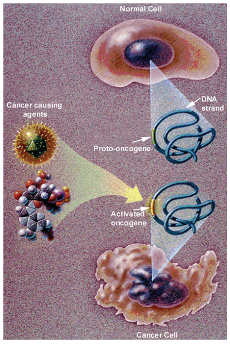
[92] | National Cancer Institute/National Institutes of Health/Department of Health and Human Services (2006) What You Need To Know About Cancer Bethesda, MD: NIH. |
[93] | Weinhouse S, Warburg O, Burk D, et al. (1956) On respiratory impairment in cancer cells. Science 124: 269–270. |
[94] | Gillies R, (2001) The Tumour Microenvironment: Causes and Consequences of Hypoxia and Acidity, Novartis Foundation Symposium 240, New York: JohnWiley & Sons. |
[95] | Stavridis J, (2008) Oxidation: the Cornerstone of Carcinogenesis, New York: Springer. |
[96] |
Grek C, Tew K (2010) Redox metabolism and malignancy. Current Opin Pharmacol 10: 362–368. doi: 10.1016/j.coph.2010.05.003
![]() |
[97] |
Fogg V, Lanning N, MacKeigan J (2011) Mitochondria in cancer: at the crossroads of life and death. Chin J Cancer 30: 526–539. doi: 10.5732/cjc.011.10018
![]() |
[98] |
Hielscher A, Gerecht S (2015) Hypoxia and free radicals: role in tumor progression and the use of engineering-based platforms to address these relationships. Free Radic Biol Med 79: 281–291. doi: 10.1016/j.freeradbiomed.2014.09.015
![]() |
[99] |
Görlach A, Dimova E, Petry A, et al. (2015) Reactive oxygen species, nutrition, hypoxia and diseases: problems solved? Redox Biol 6: 372–385. doi: 10.1016/j.redox.2015.08.016
![]() |
[100] | Tafani M, Sansone L, Limana F, et al. (2016) The interplay of reactive oxygen species, hypoxia, inflammation, and sirtuins in caner initiation and progression. Oxid Med Cell Longev 2016: 1–18. |
[101] | Peacock J, Calhoun A, (2006) Polymer Chemistry Properties and Applications, Munich, Germany: Hanser. |
[102] |
Mironi-Harpaz I, Narkis M, Siegmann A (2007) Peroxide crosslinking of a styrene-free unsaturated polyester. J Appl Polym Sci 105: 885–892. doi: 10.1002/app.25385
![]() |
[103] |
Wang Y, Woodworth L, Han B (2011) Simultaneous measurement of effective chemical shrinkage and modulus evolutions during polymerization. Exp Mech 51: 1155–1169. doi: 10.1007/s11340-010-9410-y
![]() |
[104] |
Jansen K, Vreugd de J, Ernst L (2012) Analytical estimate for curing-induced stress and warpage in coating layers. J Appl Polym Sci 126: 1623–1630. doi: 10.1002/app.36776
![]() |
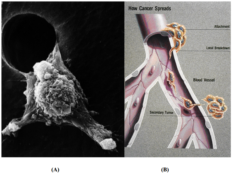
[105] | Weinberg R, (2007) 14.3 The epithelial-mesenchymal transition and associated loss of E-cadherin expression enable carcinoma cells to become invasive, In: The Biology of Cancer, New York: Garland Science, 597–624. |
[106] |
Wenger J, Chun S, Dang D, et al. (2011) Combination therapy targeting cancer metabolism. Med Hypotheses 76: 169–172. doi: 10.1016/j.mehy.2010.09.008
![]() |
[107] |
Vinogradova T, Miller P, Kaverina I (2009) Microtubule network asymmetry in motile cells: role of Golgi-derived array. Cell Cycle 8: 2168–2174. doi: 10.4161/cc.8.14.9074
![]() |
[108] |
Lindberg U, Karlsson R, Lassing I, et al. (2008) The microfilament system and malignancy. Semin Cancer Biol 18: 2–11. doi: 10.1016/j.semcancer.2007.10.002
![]() |
[109] |
San Martín A, Griendling K (2010) Redox control of vascular smooth muscle migration. Antioxid Redox Signal 12: 625–640. doi: 10.1089/ars.2009.2852
![]() |
[110] | Copstead LE, Banasik J, (2005) Pathophysiology, 6 Eds., St. Louis, MO: Elsevier Saunders, 221. |
[111] |
Li Z, Hannigan M, Mo Z, et al. (2003) Directional Sensing Requires Gβγ-Mediated PAK1 and PIXα-Dependent Activation of Cdc42. Cell 114: 215–227. doi: 10.1016/S0092-8674(03)00559-2
![]() |
[112] |
Hattori H, Subramanian K, Sakai J, et al. (2010) Small-molecule screen identifies reactive oxygen species as key regulators of neutrophile chemotaxis. PNAS 107: 3546–3551. doi: 10.1073/pnas.0914351107
![]() |
[113] |
Parisi F, Vidal M (2011) Epithelial delamination and migration: lessons from Drosophila. Cell Adh Migr 5: 366–372. doi: 10.4161/cam.5.4.17524
![]() |
[114] |
Barth A, Caro-Gonzalez H, et al. (2008) Role of adenomatous polyposis coli (APC) and microtubules in directional cell migration and neuronal polarization. Semin Cell Dev Biol 19: 245–251. doi: 10.1016/j.semcdb.2008.02.003
![]() |
[115] | Dent E, Gupton S, et al. (2010) The growth cone cytoskeleton in axon outgrowth and guidance. Cold Spring Harb Perspect Biol 3: a001800. |
[116] |
Saraswathy S, Wu G, et al. (2006) Retinal microglial activation and chemotaxis by docosahexaenoic acid hydroperoxide. Invest Ophthalmol Vis Sci 47: 3656–3663. doi: 10.1167/iovs.06-0221
![]() |
[117] |
Dunlop R, Dean R, Rodgers K (2008) The impact of specific oxidized amino acids on protein turnover in J774 cells. Biochem J 410: 131–140. doi: 10.1042/BJ20070161
![]() |
[118] |
Darling E, Zauscher S, Block J (2007) A thin-layer model for viscoelastic, stress-relaxation testing of cells using atomic force microscopy: do cell properties reflect metastatic potential. Biophys J 92: 1784–1791. doi: 10.1529/biophysj.106.083097
![]() |
[119] |
Fleischer F, Ananthakrishnan R, (2007) Actin network architecture and elasticity in lamellipodia of melanoma cells. New J Phys 9: 420. doi: 10.1088/1367-2630/9/11/420
![]() |
[120] | Pokorný J, Jandový A, Nedbalová (2012) Mitochondrial metabolism-neglected link of cancer transformation and treatment. Prague Med Rep 113: 81–94. |
[121] |
Qian Y, Luo J, Leonard S, et al. (2003) Hydrogen peroxide formation and actin filament reorganization by Cdc42 are essential for ethanol-induced in vitro angiogenesis. J Biol Chem 278: 16189–16197. doi: 10.1074/jbc.M207517200
![]() |
[122] |
Gawdzik B, Księzopolski J, Matynia T (2003) Synthesis of new free-radical initiators for polymerization. J Appl Polym Sci 87: 2238–2243. doi: 10.1002/app.11585
![]() |
[123] |
Miller Y, Worrall D, Funk C, et al. (2003) Actin polymerization in macrophages in response to oxidized LDL and apoptotic cells: role of 12/15-lipoxygenase and phosphoinositide 3-kinase. Mol Biol Cell 14: 4196–4206. doi: 10.1091/mbc.E03-02-0063
![]() |
[124] |
Ushio-Fukai M, Nakamura Y (2008) Reactive oxygen species and angiogenesis: NADPH oxidase as target for cancer therapy. Cancer Lett 266: 37–52. doi: 10.1016/j.canlet.2008.02.044
![]() |
[125] |
Taparowsky E, Suard Y, Fasano O (1982) Activation of the T24 bladder carcinoma transforming gene is linked to a single amino acid change. Nature 300: 762–765. doi: 10.1038/300762a0
![]() |
[126] |
Swaminathan V, Mythreye K, Tim O'Brien E, et al. (2011) Mechanical Stiffness grades metastatic potential in patient tumor cells and in cancer cell lines. Cancer Res 71: 5075–5080. doi: 10.1158/0008-5472.CAN-11-0247
![]() |
[127] |
Xu W, Mezencev R, Kim B, et al. (2012) Cell stiffness is a biomarker of the metastatic potential of ovarian cancer cells. PLoS ONE 7: e46609. doi: 10.1371/journal.pone.0046609
![]() |
[128] |
Hoyt K, Castaneda B, Zhang M, et al. (2008) Tissue elasticity properties as biomarkers for prostate cancer. Cancer Biomark 4: 213–225. doi: 10.3233/CBM-2008-44-505
![]() |
[129] |
Ghosh S, Kang T, Wang H, et al. (2011) Mechanical phenotype is important for stromal aromatase expression. Steroids 76: 797–801. doi: 10.1016/j.steroids.2011.02.039
![]() |
[130] |
Kraning-Rush C, Califano J, Reinhart-King C (2012) Cellular traction stresses increase with increasing metastatic potential. PLoS ONE 7: e32572. doi: 10.1371/journal.pone.0032572
![]() |
[131] | Trichet L, Le Digabel J, Hawkins R, et al. Evidence of a large-scale mechanosensing mechanism for cellular adaptation to substrate stiffness. Proc Natl Acad Sci U.S.A. 109: 6933–6938. |
[132] |
Peto R, Doll R, Buckley J (1981) Can dietary beta-carotene materially reduce human cancer rates? Nature 290: 201–208. doi: 10.1038/290201a0
![]() |
[133] | Shike M, Winawer S, Greenwald P, et al. (1990) Primary prevention of colorectal cancer. Bull World Health Organ 68: 337–385. |
[134] | Dorgan J, Schatzkin A (1991) Antioxidant micronutrients in cancer prevention. Hematol Oncol Clin North Am 5: 43–68. |
[135] |
Chlebowski R, Grosvenor M (1994) The scope of nutrition intervention trials with cancer-related endpoints. Cancer 74: 2734–2738. doi: 10.1002/1097-0142(19941101)74:9+<2734::AID-CNCR2820741824>3.0.CO;2-U
![]() |
[136] |
Ziegler R, Mayne S, Swanson C (1996) Nutrition and lung cancer. Cancer Causes Control 7: 157–177. doi: 10.1007/BF00115646
![]() |
[137] | Levander O (1997) Symposium: newly emerging viral diseases: what role for nutrition? J Nutr 127: 948S–950S. |
[138] | Willett W (1999) Convergence of philosophy and science: the Third International Congress on Vegetarian Nutrition. Am J Clin Nutr 70(suppl): 434S–438S. |
[139] | Meydani M (2000) Effect of functional food ingredients: vitamin E modulation of cardiovascular diseases and immune status in the elderly. Am J Clin Nutr 71(suppl): 1665S–1668S. |
[140] | Simopoulos A (2001) The Mediterranean diets: what is so special about the diet of Greece? The scientific experience. J Nutr 131: 3065S–3073S. |
[141] |
Rock C, Demark-Wahnefried W (2002) Nutrition and survival after the diagnosis of breast cancer: a review of the evidence. J Clin Oncol 20: 3302–3316. doi: 10.1200/JCO.2002.03.008
![]() |
[142] | Seifried H, McDonald S, Anderson D, et al. (2003) The antioxidant conundrum in cancer. Cancer Res 63: 4295–4298. |
[143] |
Männistö S, Smith-Warner S, Spiegelman D, et al. (2004) Dietary carotenoids and risk of lung cancer in a pooled analysis of seven cohort studies. Cancer Epidemiol Biomarkers Prev 13: 40–48. doi: 10.1158/1055-9965.EPI-038-3
![]() |
[144] | Fraga C (2007) Plant polyphenols: how to translate their in vitro antioxidant actions to in vivo conditions. Life 59: 308–315. |
[145] |
Kushi L, Doyle C, McCullough M, et al. (2012) American cancer society guidelines on nutrition and physical activity for cancer prevention. CA Cancer J Clin 62: 30–67. doi: 10.3322/caac.20140
![]() |
[146] |
Heinonen O, Albanes D, Huttunen J, et al. (1994) The effect of vitamin E and beta carotene on the incidence of lung cancer and other cancers in male smokers. N Engl J Med 330: 1029–1035. doi: 10.1056/NEJM199404143301501
![]() |
[147] |
Hennekens C, Buring J, Manson J, et al. (1996) Lack of effect of long-term supplementation with beta carotene on the incidence of malignant neoplasms and cardiovascular disease. N Engl J Med 334: 1145–1149. doi: 10.1056/NEJM199605023341801
![]() |
[148] |
Omenn G, Goodman G, Thornquist M, et al. (1996) Effects of a combination of beta carotene and vitamin A on lung cancer and cardiovascular disease. N Engl J Med 334: 1150–1155. doi: 10.1056/NEJM199605023341802
![]() |
[149] | Albanes D (1999) β-carotene and lung cancer: a case study. Am J Clin Nutr 69(suppl): 1345S–1350S. |
[150] |
Virtamo J, Albanes D, Huttunen J, et al. (2003) Incidence of cancer and mortality following α-tocopherol and β-carotene supplementation. JAMA 290: 476–485. doi: 10.1001/jama.290.4.476
![]() |
[151] | Sommer A, Vyas K (2012) A global clilnical view on vitamin A and carotenoids. Am J Clin Nutr 96(suppl): 1204–1206. |
[152] | Thompson I, Kristal A, Platz E (2014) Prevention of prostate cancer: outcomes of clinical trails and future opportunities. Am Soc Clin Oncol Educ Book 2014: e76–e80. |
[153] |
Virtamo J, Taylor P, Kontto J, et al (2014) Effects of α-tocopherol and β-carotene supplementation on cancer incidence and mortality: 18-year post-intervention follow-up of the alpha-tocopherol, beta-carotene cancer prevention (ATBC) study. Int J Cancer 135: 178–185. doi: 10.1002/ijc.28641
![]() |
[154] |
Yusuf S, Phil D, Dagenais G, et al. (2000) Vitamin E supplementation and cardiovascular events in high-risk patients. N Engl J Med 342: 154–160. doi: 10.1056/NEJM200001203420302
![]() |
[155] | Devaraj S, Tang R, Adams-Huet B, et al. (2007) Effect of high-dose α-tocopherol supplementation on biomarkers of oxidative stress and inflammation and carotid atherosclerosis in patients with coronary artery disease. Am J Clin Nutr 86: 1392–1398. |
[156] | Sesso H, Buring J, Christen W, et al (2008) Vitamins E and C in the prevention of cardiovascular disease in men. JAMA 300: 2123–2133. |
[157] |
Brigelius-Flohe R, Galli F (2010) Vitamin E: a vitamin still awaiting the detection of its biological function. Mol Nutr Food Res 54: 583–587. doi: 10.1002/mnfr.201000091
![]() |
[158] | Schultz M, Leist M, Petrzika M, et al. (1995) Novel urinary metabolite of α-tocopherol, 2,5,7,8-tetramethyl-2(2'-carboxyethyl)-6-hydroxychroman, as an indicator of an adequate vitamin E supply. Am J Clin Nutr 62(suppl): 1527S–1534S. |
[159] |
Azzi A (2007) Molecular mechanism of α-tocopherol action. Free Radic Biol Med 43: 16–21. doi: 10.1016/j.freeradbiomed.2007.03.013
![]() |
[160] | Boddupalli S, Mein J, Lakkanna S, et al. (2012) Induction of phase 2 antioxidant enzymes by broccoli sulforaphane: perspectives in maintaining the antioxidant activity of vitamins A, C, and E. Front Genet 3: 1–15. |
[161] |
Lü JM, Lin P, Yao Q, et al. (2010) Chemical and molecular mechanisms of antioxidants: experimental approaches and model systems. J Cell Mol Med 14: 840–860. doi: 10.1111/j.1582-4934.2009.00897.x
![]() |
[162] | Apak R, Güçlü K, Özyürek M, et al. (2008) Mechanism of antioxidant capacity assays and the CUPRAC (cupric ion reducing antioxidant capacity) assay. Microch Acta 160: 413–419. |
[163] |
Özyürek M, Bektaşoğlu B, Güçlü K, et al. (2008) Simultaneous total antioxidant capacity assay of lipohilic and hydrophilic antioxidants in the same acetone-water solution containing 2% methyl-β-cyclodextrin using the cupric reducing antioxidant capacity (CUPRAC) method. Anal Chim ACTA 630: 28–39. doi: 10.1016/j.aca.2008.09.057
![]() |
[164] | McMurry J, (2004) Organic Chemistry, 6 Eds., Belmont, CA: Thompson Brooks/Cole, 403–405, 482–483, 486–487. |
[165] |
Dumas D, Muller S, Gouin F, et al. (1997) Membrane fluidity and oxygen diffusion in cholesterol enriched erythrocyte membrane. Arch Biochem Biophys 341: 34–39. doi: 10.1006/abbi.1997.9936
![]() |
[166] |
Cazzola R, Rondanelli M, Russo-Volpe S, et al. (2004) Decreased membrane fluidity and altered susceptibility to peroxidation and lipid composition in overweight and obese female erythrocytes. J Lipid Res 45: 1846–1851. doi: 10.1194/jlr.M300509-JLR200
![]() |
[167] | Madmani M, Yusaf S, Tamr A, et al. (2014) Coenzyme Q10 for heart failure (Review). Cochrane Database Syst Rev 2014. |
[168] | Watts G, Playford D, Croft K, et al. (2002). Coenzyme Q10 improves endothelial dysfunction of brachial artery in type II diabetes mellitus. Diabetologia 45:420–426. |
[169] |
DeCaprio A (1999) The toxicology of hydroquinone-relevance to occupational and environmental exposure. Crit Rev Toxicol 29: 283–330. doi: 10.1080/10408449991349221
![]() |
[170] | McMurry J, (2004) 17.11 Reactions of Phenols, In: Organic Chemistry, 6 Eds., Belmont, CA: Thompson Brooks/Cole, 618–619. |
[171] |
Takata J, Matsunage K, Karube Y (2002) Delivery systems for antioxidant nutrients. Toxicology 180: 183–193. doi: 10.1016/S0300-483X(02)00390-6
![]() |
[172] |
Pifer, J, Hearne F, Friedlander B, et al. (1986) Mortality study of men employed at a large chemical plant, 1972 through 1982. J Occup Med 28: 438–444. doi: 10.1097/00043764-198606000-00011
![]() |
[173] |
Pifer J, Hearne F, Swanson F (1995) Mortality study of employees engaged in the manufacture and use of hydroquinone. Int Arch Occup Environ Health 67: 267–280. doi: 10.1007/BF00409409
![]() |
[174] | Sterner J, Oglesby F, Anderson B (1947) Quinone vapors and their harmful effects. I Corneal and conjunctival injury. J Ind Hyg Toxicol 29: 60–73. |
[175] |
Carlson A, Brewer N (1953) Toxicity studies on hydroquinone. Proc Soc Exp Biol Med 84: 684–688. doi: 10.3181/00379727-84-20751
![]() |
[176] |
O'Donoghue J (2006) Hydroquinone and its analogues in dermatology-a risk-benefit viewpoint. J Cosmet Dermatol 5: 196–203. doi: 10.1111/j.1473-2165.2006.00253.x
![]() |
[177] | Nordlund J, Grimes P, Ortonne J (2006) The safety of hydroquinone. JEADV 20: 781–787. |
[178] |
Arndt K, Fitzpatrick T (1965) Topical use of hydroquinone as a depigmenting agent. JAMA 194: 965–967. doi: 10.1001/jama.1965.03090220021006
![]() |
[179] | Deisinger P, Hill T, English C (1996) Human exposure to naturally occurring hydroquinone. J Toxicol Env Health 47: 31–46. |
[180] |
Levitt J (2007) The safety of hydroquinone: a dermatologist's response to the 2006 Federal Register. J Am Acad Dermatol 57: 854–872. doi: 10.1016/j.jaad.2007.02.020
![]() |
[181] |
Marcus R, Sutin N (1985) Electron transfers in chemistry and biology. Biochim Biophys Acta 811: 265–322. doi: 10.1016/0304-4173(85)90014-X
![]() |
[182] | Dumas D, Latger V, Viriot M-L, et al. (1999) Membrane fluidity and oxygen diffusion in cholesterol-enriched endothelial cells. Clin Hemorheol Microcirc 21: 255–261. |
[183] | National Toxicology Program (1989) Toxicology and carcinogenesis studies of hydroquinone in F-344/N rats and B6C3F mice. NIH Publication : 90–2821. |
[184] |
Shibata MA, Hirose M, Tanaka H, et al. (1991) Induction of renal cell tumors in rats and mice, and enhancement of hepatocellular tumor development in mice after long-term hydroquinone treatment. Jap J Can Res 82: 1211–1219. doi: 10.1111/j.1349-7006.1991.tb01783.x
![]() |
[185] |
Poet T, Wu H, English J, et al (2004) Metabolic rate constants for hydroquinone in F344 rat and human liver isolated hepatocytes: application to a PBPK model. Toxicol Sci 82: 9–25. doi: 10.1093/toxsci/kfh229
![]() |
[186] |
MacDonald J (2004) Human carcinogenic risk evaluation, part IV: assessment of human risk of cancer from chemical exposure using a global weight-of-evidence approach. Toxicol Sci 82: 3–8. doi: 10.1093/toxsci/kfh189
![]() |
[187] | Food and Drug Administration (2015) Hydroquinone studies under the national toxicology program (NTP). 11/27/2015. Accessed 11/2016, Available from: http://www.fda/gov/About FDA/CentersOffices/OfficeofMedicalProductsandTobacco/CDER/ucm203112.htm. |
1. | Guowei Sun, Ali Mai, Stability Analysis of a Two-Patch Competition Model with Dispersal Delays, 2019, 2019, 1026-0226, 1, 10.1155/2019/3159591 | |
2. | Siheng Xiao, Yuanshi Wang, Shikun Wang, Effects of Prey’s Diffusion on Predator–Prey Systems with Two Patches, 2021, 83, 0092-8240, 10.1007/s11538-021-00884-6 | |
3. | Thibault Moulin, Antoine Perasso, Ezio Venturino, A Metaecoepidemic Model of Grassland Ecosystem with Only Consumers’ Migration, 2020, 82, 0092-8240, 10.1007/s11538-020-00764-5 | |
4. | Xuejuan Lu, Yuming Chen, Shengqiang Liu, A Stage-Structured Predator-Prey Model in a Patchy Environment, 2020, 2020, 1076-2787, 1, 10.1155/2020/6028019 | |
5. | Guowei Sun, Ali Mai, Stability analysis of a two-patch predator–prey model with two dispersal delays, 2018, 2018, 1687-1847, 10.1186/s13662-018-1833-2 | |
6. | Wenbin Yang, Existence and asymptotic behavior of solutions for a mathematical ecology model with herd behavior, 2020, 43, 0170-4214, 5629, 10.1002/mma.6301 | |
7. | Kun Hu, Yuanshi Wang, Dynamics of consumer-resource systems with consumer's dispersal between patches, 2021, 0, 1553-524X, 0, 10.3934/dcdsb.2021077 | |
8. | David Brown, Andrea Bruder, Miroslav Kummel, Endogenous spatial heterogeneity in a multi-patch predator-prey system: insights from a field-parameterized model, 2020, 1874-1738, 10.1007/s12080-020-00483-6 | |
9. | Ali Mai, Guowei Sun, Fengqin Zhang, Lin Wang, The joint impacts of dispersal delay and dispersal patterns on the stability of predator-prey metacommunities, 2019, 462, 00225193, 455, 10.1016/j.jtbi.2018.11.035 | |
10. | Sangeeta Saha, G. P. Samanta, Influence of dispersal and strong Allee effect on a two-patch predator–prey model, 2019, 7, 2195-268X, 1321, 10.1007/s40435-018-0490-3 | |
11. | Ali Mai, Guowei Sun, Lin Wang, Impacts of the Dispersal Delay on the Stability of the Coexistence Equilibrium of a Two-Patch Predator–Prey Model with Random Predator Dispersal, 2019, 81, 0092-8240, 1337, 10.1007/s11538-018-00568-8 | |
12. | Guowei Sun, Ali Mai, Stability switches in a ring-structured predator–prey metapopulation model with dispersal delay, 2020, 2020, 1687-1847, 10.1186/s13662-020-02635-8 | |
13. | M.P. Kulakov, E.V. Kurilova, E.Ya. Frisman, Synchronization and Bursting Activity in the Model for Two Predator-Prey Systems Coupled By Predator Migration, 2019, 14, 19946538, 588, 10.17537/2019.14.588 | |
14. | Érika Diz-Pita, M. Victoria Otero-Espinar, Predator–Prey Models: A Review of Some Recent Advances, 2021, 9, 2227-7390, 1783, 10.3390/math9151783 | |
15. | S. Biswas, D. Pal, P. K. Santra, Ebenezer Bonyah, G. S. Mahapatra, Cruz Vargas-De-León, Dynamics of a Three-Patch Prey-Predator System with the Impact of Dispersal Speed Incorporating Strong Allee Effect on Double Prey, 2022, 2022, 1607-887X, 1, 10.1155/2022/7919952 | |
16. | A. George Maria Selvam, S. Britto Jacob, Mary Jacintha, D. Abraham Vianny, 2022, 2385, 0094-243X, 130038, 10.1063/5.0070753 | |
17. | Rina Su, Chunrui Zhang, The generation mechanism of Turing-pattern in a Tree-grass competition model with cross diffusion and time delay, 2022, 19, 1551-0018, 12073, 10.3934/mbe.2022562 | |
18. | Sangeeta Saha, Guruprasad Samanta, Impact of disease on a two-patch eco-epidemic model in presence of prey dispersal, 2022, 10, 2544-7297, 199, 10.1515/cmb-2022-0139 | |
19. | Xin Zhao, Zhijun Zeng, Stochastic Dynamics of a Two-Species Patch-System With Ratio-Dependent Functional Response, 2022, 21, 1575-5460, 10.1007/s12346-022-00594-x | |
20. | Ali Mai, Guowei Sun, Lin Wang, Effects of dispersal on competitive coexistence in a two‐patch competition model, 2023, 0170-4214, 10.1002/mma.9137 | |
21. | Tin Phan, James J. Elser, Yang Kuang, Rich Dynamics of a General Producer–Grazer Interaction Model under Shared Multiple Resource Limitations, 2023, 13, 2076-3417, 4150, 10.3390/app13074150 | |
22. | James L. L. Lichtenstein, Oswald J. Schmitz, Incorporating neurological and behavioral mechanisms of sociality into predator-prey models, 2023, 17, 1662-5153, 10.3389/fnbeh.2023.1122458 | |
23. | Yuanyuan Zhang, Dan Huang, Shanshan Chen, The Effect of Dispersal Patterns on Hopf Bifurcations in a Delayed Single Population Model, 2023, 33, 0218-1274, 10.1142/S0218127423500530 | |
24. | Yue Xia, Lijuan Chen, Vaibhava Srivastava, Rana D. Parshad, Stability and bifurcation analysis of a two-patch model with the Allee effect and dispersal, 2023, 20, 1551-0018, 19781, 10.3934/mbe.2023876 | |
25. | Minjuan Gao, Lijuan Chen, Fengde Chen, Dynamical analysis of a discrete two-patch model with the Allee effect and nonlinear dispersal, 2024, 21, 1551-0018, 5499, 10.3934/mbe.2024242 | |
26. | Min Lu, Chuang Xiang, Jicai Huang, Shigui Ruan, Dynamics of the generalized Rosenzweig–MacArthur model in a changing and patchy environment, 2024, 01672789, 134197, 10.1016/j.physd.2024.134197 | |
27. | Animesh Samanta, Tapan Chatterjee, Priyanka Mandal, Ayan Chatterjee, Madan Kumar Jha, Mritunjay Kumar Singh, Modeling Saltwater Intrusion into Groundwater Using a Prey–Predator Model, 2024, 29, 1084-0699, 10.1061/JHYEFF.HEENG-6071 | |
28. | Deeptajyoti Sen, Lenka Přibylová, Complex dynamics in prey-predator systems with cross-coupling: Exploring nonlinear interactions and population oscillations, 2024, 10075704, 108154, 10.1016/j.cnsns.2024.108154 | |
29. | Hasan S. Panigoro, Emli Rahmi, Olumuyiwa James Peter, 2024, 3083, 0094-243X, 050003, 10.1063/5.0224886 | |
30. | Bapan Ghosh, Dispersal induced catastrophic bifurcations, Arnold tongues, shrimp structures, and stock patterns in an ecological system, 2024, 34, 1054-1500, 10.1063/5.0240974 | |
31. | Debjani Mondal, Moitri Sen, Deeptajyoti Sen, Exploring population oscillations: Cross-coupling and dispersal effects in prey-predator dynamics, 2025, 01672789, 134525, 10.1016/j.physd.2025.134525 | |
32. | Lucero Rodriguez Rodriguez, Marisabel Rodriguez Messan, Komi Messan, Yun Kang, Mathematical modeling of natural resource and human interaction: Applications to the harvesting of Pacific Yew for cancer treatment, 2025, 0, 2155-3289, 0, 10.3934/naco.2025003 | |
33. | Jin Zhong, Yue Xia, Lijuan Chen, Fengde Chen, Dynamical analysis of a predator-prey system with fear-induced dispersal between patches, 2025, 22, 1551-0018, 1159, 10.3934/mbe.2025042 | |
34. | Sangeeta Kumari, Sidharth Menon, Abhirami K, Dynamical system of quokka population depicting Fennecaphobia by Vulpes vulpes, 2025, 22, 1551-0018, 1342, 10.3934/mbe.2025050 |
Scenarios | Model (4) whose dispersal is driven by the strength of prey-predator interactions | Classical Model (12) whose dispersal is driven by the density of predators |
LAS and GAS if |
GAS if |
|
LAS if |
Does not exists | |
Does not exists | LAS if |
Scenarios | Model (4) whose dispersal is driven by the strength of prey-predator interactions | Classical Model (12) whose dispersal is driven by the density of predators |
Persistence of prey | Always persist, dispersal of predator has no effects | One or both prey persist if conditions 4. in Theorem (4.1) holds. Small dispersal of predator in Patch |
Extinction of prey | Never extinct |
Scenarios | Model (4) whose dispersal is driven by the strength of prey-predator interactions | Classical Model (12) whose dispersal is driven by the density of predators |
Persistence of predator | Predator at Patch |
Predators in both patches have the same persistence conditions. They persist if |
Extinction of predator | Simulations suggestions (see the yellow regions of Figure (1a) and Figure (3a)) that the large dispersal of predator in Patch |
Predators in both patches have the same extinction conditions. They go extinct if |
Scenarios | Model (4) whose dispersal is driven by the strength of prey-predator interactions | Classical Model (12) whose dispersal is driven by the density of predators |
LAS and GAS if |
GAS if |
|
LAS if |
Does not exists | |
Does not exists | LAS if |
Scenarios | Model (4) whose dispersal is driven by the strength of prey-predator interactions | Classical Model (12) whose dispersal is driven by the density of predators |
Persistence of prey | Always persist, dispersal of predator has no effects | One or both prey persist if conditions 4. in Theorem (4.1) holds. Small dispersal of predator in Patch |
Extinction of prey | Never extinct |
Scenarios | Model (4) whose dispersal is driven by the strength of prey-predator interactions | Classical Model (12) whose dispersal is driven by the density of predators |
Persistence of predator | Predator at Patch |
Predators in both patches have the same persistence conditions. They persist if |
Extinction of predator | Simulations suggestions (see the yellow regions of Figure (1a) and Figure (3a)) that the large dispersal of predator in Patch |
Predators in both patches have the same extinction conditions. They go extinct if |