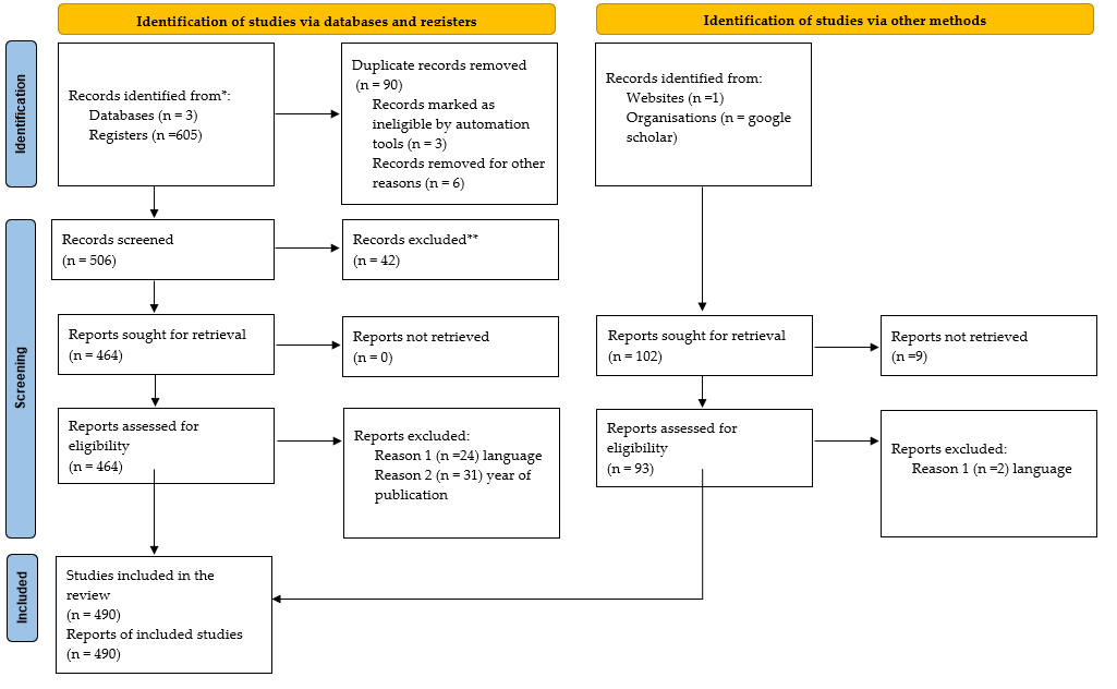
Insurance companies are responding to the global challenge of climate change by introducing green insurance policies, which aim to promote sustainable projects across the globe. These policies offer financial protection and coverage for initiatives related to renewable energy, energy efficiency and other sustainable endeavors. Moreover, they incentivize investment in these projects by providing lower premiums or other financial benefits. In order to assess the impact of green insurance policies on driving investment in sustainable projects in developing countries, this study employed a systematic and bibliometric approach to thoroughly analyze the various forms, instruments, and measurements of green insurance. The study used 490 documents extracted from different databases. The search strategy involved using specific keywords to query the Web of Science, Scopus, science direct, and google scholar databases. A purposive sampling technique was implemented for data inclusion and exclusion. The study's findings indicate that the success of green insurance in developing countries faces several challenges, including inadequate infrastructure, limited awareness and education among individuals and businesses, absence of supportive regulatory frameworks and policies, insufficient demand, political instability, corruption and security concerns. Furthermore, the study finding reveals a need for more research, specifically exploring the effects of green insurance on investment in sustainable development. Hence future studies can use this finding as a benchmark for further studies. The study's novelty lies in its comprehensive analysis of green insurance policies and their impact on driving investment in sustainable projects in developing countries. Based on the findings, the study recommends that insurance companies offer incentives to investors involved in sustainable projects, such as employing premium shifting strategies that minimize premiums for non-environmentally sustainable projects and redirect those funds toward sustainable initiatives.
Citation: Goshu Desalegn. Insuring a greener future: How green insurance drives investment in sustainable projects in developing countries?[J]. Green Finance, 2023, 5(2): 195-210. doi: 10.3934/GF.2023008
Insurance companies are responding to the global challenge of climate change by introducing green insurance policies, which aim to promote sustainable projects across the globe. These policies offer financial protection and coverage for initiatives related to renewable energy, energy efficiency and other sustainable endeavors. Moreover, they incentivize investment in these projects by providing lower premiums or other financial benefits. In order to assess the impact of green insurance policies on driving investment in sustainable projects in developing countries, this study employed a systematic and bibliometric approach to thoroughly analyze the various forms, instruments, and measurements of green insurance. The study used 490 documents extracted from different databases. The search strategy involved using specific keywords to query the Web of Science, Scopus, science direct, and google scholar databases. A purposive sampling technique was implemented for data inclusion and exclusion. The study's findings indicate that the success of green insurance in developing countries faces several challenges, including inadequate infrastructure, limited awareness and education among individuals and businesses, absence of supportive regulatory frameworks and policies, insufficient demand, political instability, corruption and security concerns. Furthermore, the study finding reveals a need for more research, specifically exploring the effects of green insurance on investment in sustainable development. Hence future studies can use this finding as a benchmark for further studies. The study's novelty lies in its comprehensive analysis of green insurance policies and their impact on driving investment in sustainable projects in developing countries. Based on the findings, the study recommends that insurance companies offer incentives to investors involved in sustainable projects, such as employing premium shifting strategies that minimize premiums for non-environmentally sustainable projects and redirect those funds toward sustainable initiatives.

| [1] |
Belozyorov SA, Xie X (2021) China's green insurance system and functions. E3S Web of Conferences, 311. https://doi.org/10.1051/e3sconf/202131103001 doi: 10.1051/e3sconf/202131103001

|
| [2] | Christiansen J (2021) Securing the sea: ecosystem-based adaptation and the biopolitics of insuring nature's rents. J Polit Ecol 28: 337–357. |
| [3] |
Collier SJ, Elliott R, Lehtonen TK (2021) Climate change and insurance. Econ Soc 50: 158–172. https://doi.org/10.1080/03085147.2021.1903771 doi: 10.1080/03085147.2021.1903771
|
| [4] |
Green TL, Kronenberg J, Andersson E, et al. (2016) Insurance Value of Green Infrastructure in and Around Cities. Ecosystems 19: 1051–1063. https://doi.org/10.1007/s10021-016-9986-x doi: 10.1007/s10021-016-9986-x
|
| [5] |
Hafner S, Jones A, Anger-Kraavi A, et al. (2020) Closing the green finance gap—A systems perspective. Environ Innov Soc TR 34: 26–60. https://doi.org/10.1016/j.eist.2019.11.007 doi: 10.1016/j.eist.2019.11.007
|
| [6] | Hazell P, Anderson J, Balzer N, et al. (2010) The potential for scale and sustainability in weather index insurance for agriculture and rural livelihoods. World Food Programme (WFP). |
| [7] |
Hou D, Wang X (2022) Inhibition or Promotion?—The Effect of Agricultural Insurance on Agricultural Green Development. Front Public Health 10. https://doi.org/10.3389/fpubh.2022.910534 doi: 10.3389/fpubh.2022.910534
|
| [8] |
Johnson L (2021) Rescaling index insurance for climate and development in Africa. Econ Soc 50: 248–274. https://doi.org/10.1080/03085147.2020.1853364 doi: 10.1080/03085147.2020.1853364
|
| [9] |
Kalfin Sukono, Supian S, Mamat M (2022) Insurance as an Alternative for Sustainable Economic Recovery after Natural Disasters: A Systematic Literature Review. Sustainability 14. https://doi.org/10.3390/su14074349 doi: 10.3390/su14074349
|
| [10] | Kaminker C, Stewart F (2012) The role of institutional investors in financing clean energy. OECD Working Papers. Available from: https://www.oecd-ilibrary.org/finance-and-investment/the-role-of-institutional-investors-in-financing-clean-energy_5k9312v21l6f-en. |
| [11] |
Kassinis G, Panayiotou A (2018) Visuality as Greenwashing: The Case of BP and Deepwater Horizon. Organ Environt 31: 25–47. https://doi.org/10.1177/1086026616687014 doi: 10.1177/1086026616687014
|
| [12] |
Mills E (2003) The insurance and risk management industries: new players in the delivery of energy-efficient and renewable energy products and services. Energy Policy 31: 1257–1272. https://doi.org/10.1016/S0301-4215(02)00186-6 doi: 10.1016/S0301-4215(02)00186-6
|
| [13] |
Mills E (2009) A global review of insurance industry responses to climate change. Geneva Pap Risk Insur Issues Pract 34: 323–359. https://doi.org/10.1057/gpp.2009.14 doi: 10.1057/gpp.2009.14
|
| [14] |
Moser SC (2010) Communicating climate change: history, challenges, process and future directions. Wires Clim Change 1: 31–53. https://doi.org/10.1002/wcc.11 doi: 10.1002/wcc.11
|
| [15] | Mosley P, Garikipati S, Horrell S, et al. (2003) Risk and underdevelopment Risk management options and their significance for poverty reduction Constituent project in DFID Programme on Pro-Poor Growth (R7614/7615/7617): Risks, Incentives and Pro-Poor Growth. |
| [16] |
Nobanee H, Alqubaisi GB, Alhameli A, et al. (2021) Green and Sustainable Life Insurance: A Bibliometric Review. J Risk Financ Manage 14: 563. https://doi.org/10.3390/jrfm14110563 doi: 10.3390/jrfm14110563
|
| [17] |
Pugnetti C, Wagner J, Zeier Röschmann A (2022) Green Insurance: A Roadmap for Executive Management. J Risk Financ Manage 15: 221. https://doi.org/10.3390/jrfm15050221 doi: 10.3390/jrfm15050221
|
| [18] |
Puschmann T, Hoffmann CH, Khmarskyi V (2020) How green fintech can alleviate the impact of climate change—The case of Switzerland. Sustainability 12: 1–28. https://doi.org/10.3390/su122410691 doi: 10.3390/su122410691
|
| [19] |
Rajesh KJC, Majid MA (2020) Renewable energy for sustainable development in India: current status, future prospects, challenges, employment, and investment opportunities. Energy Sustain Soc 10. https://doi.org/10.1186/s13705-019-0232-1 doi: 10.1186/s13705-019-0232-1
|
| [20] |
Stepanova MN (2021) The place and role of insurance in shaping a "green" economy. Vestnik Universiteta 10: 147–154. https://doi.org/10.26425/1816-4277-2021-10-147-154 doi: 10.26425/1816-4277-2021-10-147-154
|
| [21] | Sussman FG (2008) Adapting to climate change: A Business approach. |
| [22] |
Vyas S, Dalhaus T, Kropff M, et al. (2021) Mapping global research on agricultural insurance. Environ Res Lett 16: 103003. https://doi.org/10.1088/1748-9326/ac263d doi: 10.1088/1748-9326/ac263d
|
| [23] |
Yang YXO, Chew BC, Loo HS, et al. (2017) Green commercial building insurance in Malaysia. AIP Conference Proceedings, 1818: 020071. https://doi.org/10.1063/1.4976935 doi: 10.1063/1.4976935
|


Figures(7) / Tables(1)

Goshu Desalegn. Insuring a greener future: How green insurance drives investment in sustainable projects in developing countries?[J]. Green Finance, 2023, 5(2): 195-210. doi: 10.3934/GF.2023008


 DownLoad: