Decision support system based on complex T-Spherical fuzzy power aggregation operators

Muhammad Qiyas; Muhammad Naeem; Saleem Abdullah; Neelam Khan; Muhammad Qiyas; Muhammad Naeem; Saleem Abdullah; Neelam Khan

doi:10.3934/math.2022884

AIMS Mathematics

2022, Volume 7, Issue 9: 16171-16207. doi: 10.3934/math.2022884

Previous Article Next Article

Research article

Decision support system based on complex T-Spherical fuzzy power aggregation operators

1.
Department of Mathematics, Abdul Wali Khan University Mardan, Mardan, KP, Pakistan
2.
Deanship of Combined First Year Umm Al-Qura University, Makkah, P.O. Box 715, Saudi Arabia

Received: 21 February 2022 Revised: 09 June 2022 Accepted: 22 June 2022 Published: 01 July 2022
MSC : 03E72, 47S40

The goal of this research is to develop many aggregation operators for aggregating various complex T-Spherical fuzzy sets (CT-SFSs). Existing fuzzy set theory and its extensions, which are a subset of real numbers, handle the uncertainties in the data, but they may lose some useful information and so affect the decision results. Complex Spherical fuzzy sets handle two-dimensional information in a single set by covering uncertainty with degrees whose ranges are extended from the real subset to the complex subset with unit disk. Thus, motivated by this concept, we developed certain CT-SFS operation laws and then proposed a series of novel averaging and geometric power aggregation operators. The properties of some of these operators are investigated. A multi-criteria group decision-making approach is also developed using these operators. The method's utility is demonstrated with an example of how to choose the best choices, which is then tested by comparing the results to those of other approaches.
- power aggregation operators,
- complex T-Spherical fuzzy sets,
- complex T-Spherical fuzzy power aggregation operators,
- decision making
Citation: Muhammad Qiyas, Muhammad Naeem, Saleem Abdullah, Neelam Khan. Decision support system based on complex T-Spherical fuzzy power aggregation operators[J]. AIMS Mathematics, 2022, 7(9): 16171-16207. doi: 10.3934/math.2022884

Related Papers:

Abstract

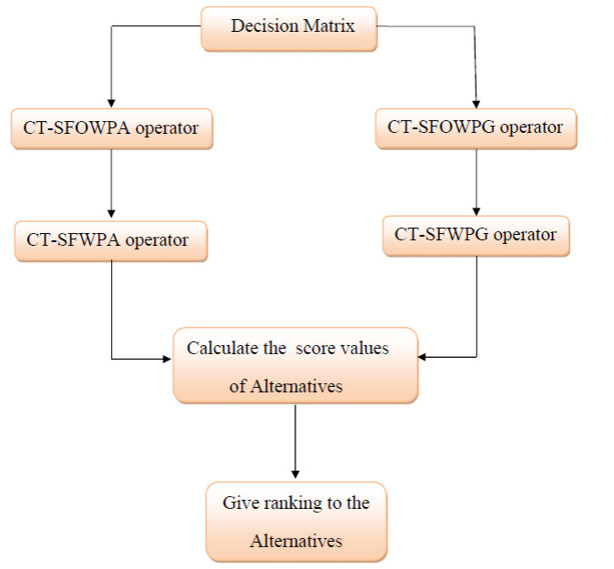
The goal of this research is to develop many aggregation operators for aggregating various complex T-Spherical fuzzy sets (CT-SFSs). Existing fuzzy set theory and its extensions, which are a subset of real numbers, handle the uncertainties in the data, but they may lose some useful information and so affect the decision results. Complex Spherical fuzzy sets handle two-dimensional information in a single set by covering uncertainty with degrees whose ranges are extended from the real subset to the complex subset with unit disk. Thus, motivated by this concept, we developed certain CT-SFS operation laws and then proposed a series of novel averaging and geometric power aggregation operators. The properties of some of these operators are investigated. A multi-criteria group decision-making approach is also developed using these operators. The method's utility is demonstrated with an example of how to choose the best choices, which is then tested by comparing the results to those of other approaches.

References

[1]	K. T. Atanassov, More on intuitionistic fuzzy sets, Fuzzy Set. Syst., 33 (1989), 37–45. https://doi.org/10.1016/0165-0114(89)90215-7 doi: 10.1016/0165-0114(89)90215-7
[2]	Z. Ali, T. Mahmood, M. S. Yang, Complex T-spherical fuzzy aggregation operators with application to multi-attribute decision making, Symmetry, 12 (2020), 1311. https://doi.org/10.3390/sym12081311 doi: 10.3390/sym12081311
[3]	M. Akram, A. Khan, J. C. R. Alcantud, G. Santos-García, A hybrid decision-making framework under complex spherical fuzzy prioritized weighted aggregation operators, Expert Syst., 38 (2021), 12712. https://doi.org/10.1111/exsy.12712 doi: 10.1111/exsy.12712
[4]	M. Akram, C. Kahraman, K. Zahid, Extension of TOPSIS model to the decision-making under complex spherical fuzzy information, Soft Comput., 25 (2021), 10771–10795. https://doi.org/10.1007/s00500-021-05945-5 doi: 10.1007/s00500-021-05945-5
[5]	M. Akram, M. Shabir, A. N. Al-Kenani, J. C. R. Alcantud, Hybrid decision-making frameworks under complex spherical fuzzy-soft sets, J. Math., 2021. https://doi.org/10.1155/2021/5563215 doi: 10.1155/2021/5563215
[6]	M. Akram, A. Khan, F. Karaaslan, Complex spherical dombi fuzzy aggregation operators for decision-making, Soft Comput., 37 (2021).
[7]	S. Abdullah, M. Qiyas, M. Naeem, Y. Liu, Pythagorean Cubic fuzzy Hamacher aggregation operators and their application in green supply selection problem, AIMS Math., 7 (2022), 4735–4766. https://doi.org/10.3934/math.2022263 doi: 10.3934/math.2022263
[8]	L. Bi, S. Dai, B. Hu, Complex fuzzy geometric aggregation operators, Symmetry, 10 (2018), 251. https://doi.org/10.3390/sym10070251 doi: 10.3390/sym10070251
[9]	Y. Chen, M. Munir, T. Mahmood, A. Hussain, S. Zeng, Some generalized T-spherical and group-generalized fuzzy geometric aggregation operators with application in MADM problems, J. Math., 2021. https://doi.org/10.1155/2021/5578797 doi: 10.1155/2021/5578797
[10]	Z. S. Chen, L. L. Yang, R. M. Rodríguez, S. H. Xiong, K. S. Chin, L. Martínez, Power-average-operator-based hybrid multiattribute online product recommendation model for consumer decision-making, Int. J. Intell. Syst., 36 (2021), 2572–2617. https://doi.org/10.1002/int.22394 doi: 10.1002/int.22394
[11]	S. Dick, R. R. Yager, O. Yazdanbakhsh, On Pythagorean and complex fuzzy set operations, IEEE T. Fuzzy Syst., 24 (2015), 1009–1021. https://doi.org/10.1109/TFUZZ.2015.2500273 doi: 10.1109/TFUZZ.2015.2500273
[12]	H. Garg, M. Munir, K. Ullah, T. Mahmood, N. Jan, Algorithm for T-spherical fuzzy multi-attribute decision making based on improved interactive aggregation operators, Symmetry, 10 (2018), 670. https://doi.org/10.3390/sym10120670 doi: 10.3390/sym10120670
[13]	H. Garg, D. Rani, Some generalized complex intuitionistic fuzzy aggregation operators and their application to multicriteria decision-making process, Arab. J. Sci. Eng., 44 (2019), 2679–2698. https://doi.org/10.1007/s13369-018-3413-x doi: 10.1007/s13369-018-3413-x
[14]	H. Garg, D. Rani, New generalised Bonferroni mean aggregation operators of complex intuitionistic fuzzy information based on Archimedean t-norm and t-conorm, J. Exp. Theor. Artif. In., 32 (2020), 81–109. https://doi.org/10.1080/0952813X.2019.1620871 doi: 10.1080/0952813X.2019.1620871
[15]	H. Garg, D. Rani, Robust averaging-geometric aggregation operators for complex intuitionistic fuzzy sets and their applications to MCDM process, Arab. J. Sci. Eng., 45 (2020), 2017–2033. https://doi.org/10.1007/S13369-019-03925-4 doi: 10.1007/S13369-019-03925-4
[16]	H. Garg, J. Gwak, T. Mahmood, Z. Ali, Power aggregation operators and VIKOR methods for complex q-rung orthopair fuzzy sets and their applications, Mathematics, 8 (2020), 538. https://doi.org/10.3390/math8040538 doi: 10.3390/math8040538
[17]	A. Guleria, R. K. Bajaj, T-spherical fuzzy soft sets and its aggregation operators with application in decision-making, Sci. Iran., 28 (2021), 1014–1029. https://doi.org/10.24200/SCI.2019.53027.3018 doi: 10.24200/SCI.2019.53027.3018
[18]	B. Hu, L. Bi, S. Dai, S. Li, Distances of complex fuzzy sets and continuity of complex fuzzy operations, J. Intell. Fuzzy Syst., 35 (2018), 2247–2255. https://doi.org/10.3233/JIFS-172264 doi: 10.3233/JIFS-172264
[19]	Y. Ju, Y. Liang, C. Luo, P. Dong, E. D. S. Gonzalez, A. Wang, T-spherical fuzzy TODIM method for multi-criteria group decision-making problem with incomplete weight information, Soft Comput., 25 (2021), 2981–3001. https://doi.org/10.1007/s00500-020-05357-x doi: 10.1007/s00500-020-05357-x
[20]	G. J. Klir, B. Yuan, Fuzzy sets and fuzzy logic: Theory and applications, prentice hall of India Private Limited, New Delhi, 2005. https://doi.org/10.5860/choice.33-2786
[21]	A. A. Khan, S. Ashraf, S. Abdullah, M. Qiyas, J. Luo, S. U. Khan, Pythagorean fuzzy Dombi aggregation operators and their application in decision support system, Symmetry, 11 (2019), 383. https://doi.org/10.3390/sym11030383 doi: 10.3390/sym11030383
[22]	F. Karaaslan, M. A. D. Dawood, Complex T-spherical fuzzy Dombi aggregation operators and their applications in multiple-criteria decision-making, Complex Intell. Syst., 2021, 1–24. https://doi.org/10.1007/s40747-021-00446-2 doi: 10.1007/s40747-021-00446-2
[23]	P. Liu, Multiple attribute group decision making method based on interval-valued intuitionistic fuzzy power Heronian aggregation operators, Comput. Ind. Eng., 108 (2017), 199–212. https://doi.org/10.1016/j.cie.2017.04.033 doi: 10.1016/j.cie.2017.04.033
[24]	P. Liu, H. Li, Interval-valued intuitionistic fuzzy power Bonferroni aggregation operators and their application to group decision making, Cogn. Comput., 9 (2017), 494–512. https://doi.org/10.1007/s12559-017-9453-9 doi: 10.1007/s12559-017-9453-9
[25]	P. Liu, P. Wang, Some q-rung orthopair fuzzy aggregation operators and their applications to multiple-attribute decision making, Int. J. Intell. Syst., 33 (2018), 259–280. https://doi.org/10.1002/int.21927 doi: 10.1002/int.21927
[26]	L. Liu, X. Zhang, Comment on Pythagorean and complex fuzzy set operations, IEEE T. Fuzzy Syst., 26 (2018), 3902–3904. https://doi.org/10.1109/TFUZZ.2018.2853749 doi: 10.1109/TFUZZ.2018.2853749
[27]	P. Liu, Q. Khan, T. Mahmood, N. Hassan, T-spherical fuzzy power Muirhead mean operator based on novel operational laws and their application in multi-attribute group decision making, IEEE Access, 7 (2019), 22613–22632. https://doi.org/10.1109/ACCESS.2019.2896107 doi: 10.1109/ACCESS.2019.2896107
[28]	P. Liu, T. Mahmood, Z. Ali, Complex q-rung orthopair fuzzy aggregation operators and their applications in multi-attribute group decision making, Information, 11 (2020), 5. https://doi.org/10.3390/info11010005 doi: 10.3390/info11010005
[29]	P. Liu, Z. Ali, T. Mahmood, Novel complex T-spherical fuzzy 2-tuple linguistic muirhead mean aggregation operators and their application to multi-attribute decision-making, Int. J. Comput. Intell. Syst., 14 (2020), 295–331. https://doi.org/10.2991/ijcis.d.201207.003 doi: 10.2991/ijcis.d.201207.003
[30]	J. Ma, G. Zhang, J. Lu, A method for multiple periodic factor prediction problems using complex fuzzy sets, IEEE T. Fuzzy Syst., 20 (2011), 32–45. https://doi.org/10.1109/TFUZZ.2011.2164084 doi: 10.1109/TFUZZ.2011.2164084
[31]	M. Munir, H. Kalsoom, K. Ullah, T. Mahmood, Y. M. Chu, T-spherical fuzzy Einstein hybrid aggregation operators and their applications in multi-attribute decision making problems, Symmetry, 12 (2020), 365. https://doi.org/10.3390/sym12030365 doi: 10.3390/sym12030365
[32]	H. T. Nguyen, A. Kandel, V. Kreinovich, Complex fuzzy sets: Towards new foundations, Ninth IEEE Int. Conf. Fuzzy Syst. FUZZ-IEEE 2000. https://doi.org/10.1109/FUZZY.2000.839195
[33]	M. Naeem, M. Qiyas, M. M. Al-Shomrani, S. Abdullah, Similarity measures for fractional orthotriple fuzzy sets using cosine and cotangent functions and their application in accident emergency response, Mathematics, 8 (2020), 1653. https://doi.org/10.3390/math8101653 doi: 10.3390/math8101653
[34]	M. Naeem, M. Qiyas, T. Botmart, S. Abdullah, N. Khan, Complex spherical fuzzy decision support system based on entropy measure and power operator, J. Funct. Space., 2022. https://doi.org/10.1155/2022/8315733 doi: 10.1155/2022/8315733
[35]	X. Peng, J. Dai, H. Garg, Exponential operation and aggregation operator for q-rung orthopair fuzzy set and their decision-making method with a new score function, Int. J. Intell. Syst., 33 (2018), 2255–2282. https://doi.org/10.1002/int.22028 doi: 10.1002/int.22028
[36]	S. G. Quek, G. Selvachandran, B. Davvaz, M. Pal, The algebraic structures of complex intuitionistic fuzzy soft sets associated with groups and subgroups, Sci. Iran., 26 (2019), 1898–1912. https://doi.org/10.24200/SCI.2018.50050.1485 doi: 10.24200/SCI.2018.50050.1485
[37]	S. G. Quek, G. Selvachandran, M. Munir, T. Mahmood, K. Ullah, L. H. Son, et al., Multi-attribute multi-perception decision-making based on generalized T-spherical fuzzy weighted aggregation operators on neutrosophic sets, Mathematics, 7 (2019), 780. https://doi.org/10.3390/math7090780 doi: 10.3390/math7090780
[38]	M. Qiyas, S. Abdullah, F. Khan, M. Naeem, Banzhaf-Choquet-Copula-based aggregation operators for managing fractional orthotriple fuzzy information, Alex. Eng. J., 61 (2022), 4659–4677. https://doi.org/10.1016/j.aej.2021.10.029 doi: 10.1016/j.aej.2021.10.029
[39]	M. Qiyas, M. Naeem, S. Abdullah, F. Khan, N. Khan, H. Garg, Fractional orthotriple fuzzy rough Hamacher aggregation operators and their application on service quality of wireless network selection, Alex. Eng. J., 61 (2022), 10433–10452. https://doi.org/10.1016/j.aej.2022.03.002 doi: 10.1016/j.aej.2022.03.002
[40]	D. Ramot, R. Milo, M. Friedman, A. Kandel, Complex fuzzy sets, IEEE T. Fuzzy Syst., 10 (2002), 171–186. https://doi.org/10.1109/91.995119 doi: 10.1109/91.995119
[41]	D. Rani, H. Garg, Complex intuitionistic fuzzy power aggregation operators and their applications in multicriteria decision-making, Expert Syst., 35 (2018), 12325. https://doi.org/10.1111/exsy.12325 doi: 10.1111/exsy.12325
[42]	G. Selvachandran, H. Garg, M. H. Alaroud, A. R. Salleh, Similarity measure of complex vague soft sets and its application to pattern recognition, Int. J. Fuzzy Syst., 20 (2018), 1901–1914. https://doi.org/10.1007/s40815-018-0492-5 doi: 10.1007/s40815-018-0492-5
[43]	P. K. Singh, G. Selvachandran, C. A. Kumar, Interval-valued complex fuzzy concept lattice and its granular decomposition, Recent Dev. Mach. Learn. Data Anal., 2019,275–283. https://doi.org/10.1007/978-981-13-1280-9_26 doi: 10.1007/978-981-13-1280-9_26
[44]	Z. Tao, B. Han, H. Chen, On intuitionistic fuzzy copula aggregation operators in multiple-attribute decision making, Cogn. Comput., 10 (2018), 610–624. https://doi.org/10.1007/s12559-018-9545-1 doi: 10.1007/s12559-018-9545-1
[45]	K. Ullah, T. Mahmood, N. Jan, Similarity measures for T-spherical fuzzy sets with applications in pattern recognition, Symmetry, 10 (2018), 193. https://doi.org/10.3390/sym10060193 doi: 10.3390/sym10060193
[46]	K. Ullah, T. Mahmood, Z. Ali, N. Jan, On some distance measures of complex Pythagorean fuzzy sets and their applications in pattern recognition, Complex Intell. Syst., 2019, 1–13. https://doi.org/10.1007/s40747-019-0103-6 doi: 10.1007/s40747-019-0103-6
[47]	K. Ullah, N. Hassan, T. Mahmood, N. Jan, M. Hassan, Evaluation of investment policy based on multi-attribute decision-making using interval valued T-spherical fuzzy aggregation operators, Symmetry, 11 (2019), 357. https://doi.org/10.3390/sym11030357 doi: 10.3390/sym11030357
[48]	K. Ullah, T. Mahmood, Z. Ali, N. Jan, On some distance measures of complex Pythagorean fuzzy sets and their applications in pattern recognition, Complex Intell. Syst., 6 (2020), 15–27. https://doi.org/10.1007/s40747-019-0103-6 doi: 10.1007/s40747-019-0103-6
[49]	K. Ullah, H. Garg, T. Mahmood, N. Jan, Z. Ali, Correlation coefficients for T-spherical fuzzy sets and their applications in clustering and multi-attribute decision making, Soft Comput., 24 (2020), 1647–1659. https://doi.org/10.1007/s00500-019-03993-6 doi: 10.1007/s00500-019-03993-6
[50]	X. Wang, E. Triantaphyllou, Ranking irregularities when evaluating alternatives by using some ELECTRE methods, Omega, 36 (2008), 45–63. https://doi.org/10.1016/j.omega.2005.12.003 doi: 10.1016/j.omega.2005.12.003
[51]	G. Wei, M. Lu, Pythagorean fuzzy power aggregation operators in multiple attribute decision making, Int. J. Intell. Syst., 33 (2018), 169–186. https://doi.org/10.1002/int.21946 doi: 10.1002/int.21946
[52]	Z. Xu, R. R. Yager, Power-geometric operators and their use in group decision making, IEEE T. Fuzzy Syst., 18 (2009), 94–105. https://doi.org/10.1109/TFUZZ.2009.2036907 doi: 10.1109/TFUZZ.2009.2036907
[53]	Z. Xu, Approaches to multiple attribute group decision making based on intuitionistic fuzzy power aggregation operators, Knowl.-Based Syst., 24 (2011), 749–760. https://doi.org/10.1016/j.knosys.2011.01.011 doi: 10.1016/j.knosys.2011.01.011
[54]	Z. Xu, X. Cai, Uncertain power average operators for aggregating interval fuzzy preference relations, Group Decis. Negot., 21 (2012), 381–397. https://doi.org/10.1007/s10726-010-9213-7 doi: 10.1007/s10726-010-9213-7
[55]	S. H. Xiong, Z. S. Chen, J. P.Chang, K. S. Chin, On extended power average operators for decision-making: A case study in emergency response plan selection of civil aviation, Comput. Ind. Eng., 130 (2019), 258–271. https://doi.org/10.1016/j.cie.2019.02.027 doi: 10.1016/j.cie.2019.02.027
[56]	R. R. Yager, The power average operator, IEEE T. Syst., 31 (2013), 724–731. https://doi.org/10.1109/3468.983429 doi: 10.1109/3468.983429
[57]	R. R. Yager, A. M. Abbasov, Pythagorean membership grades, complex numbers, and decision making, Int. J. Intell. Syst., 28 (2013), 436–452. https://doi.org/10.1002/int.21584 doi: 10.1002/int.21584
[58]	R. R. Yager, Pythagorean fuzzy subsets, 2013 joint IFSA world congress and NAFIPS annual meeting (IFSA/NAFIPS), 2013, 57–61. https://doi.org/10.1109/IFSA-NAFIPS.2013.6608375
[59]	R. R. Yager, Generalized orthopair fuzzy sets, IEEE T. Fuzzy Syst., 25 (2016), 1222–1230. https://doi.org/10.1109/TFUZZ.2016.2604005 doi: 10.1109/TFUZZ.2016.2604005
[60]	Z. Yang, X. Li, H. Garg, M. Qi, Decision support algorithm for selecting an antivirus mask over COVID-19 pandemic under spherical normal fuzzy environment, Int. J. Environ. Res. Pub. Heal., 17 (2020), 3407. https://doi.org/10.3390/ijerph17103407 doi: 10.3390/ijerph17103407
[61]	L. A. Zadeh, Fuzzy sets, Inf. Control, 8 (2020), 338–353. https://doi.org/10.2307/2272014 doi: 10.2307/2272014
[62]	G. Zhang, T. S. Dillon, K. Y. Cai, J. Ma, J. Lu, Operation properties and $\delta $-equalities of complex fuzzy sets, Int. J. Approx. Reason., 50 (2009), 1227–1249. https://doi.org/10.1016/j.ijar.2009.05.010 doi: 10.1016/j.ijar.2009.05.010
[63]	L. Zhou, H. Chen, J. Liu, Generalized power aggregation operators and their applications in group decision making, Comput. Ind. Eng., 62 (2012), 989–999. https://doi.org/10.1016/j.cie.2011.12.025 doi: 10.1016/j.cie.2011.12.025
[64]	L. Zhou, H. Chen, A generalization of the power aggregation operators for linguistic environment and its application in group decision making, Knowl.-Based Syst., 26 (2012), 216–224. https://doi.org/10.1016/j.knosys.2011.08.004 doi: 10.1016/j.knosys.2011.08.004
[65]	L. Zhou, H. Chen, J. Liu, Generalized power aggregation operators and their applications in group decision making, Comput. Ind. Eng., 62 (2012), 989–999. https://doi.org/10.1016/j.cie.2011.12.025 doi: 10.1016/j.cie.2011.12.025
[66]	Z. Zhang, Hesitant fuzzy power aggregation operators and their application to multiple attribute group decision making, Inf. Sci., 234 (2013), 150–181. https://doi.org/10.1016/j.ins.2013.01.002 doi: 10.1016/j.ins.2013.01.002

Reader Comments

Your name:*

Email:*
© 2022 the Author(s), licensee AIMS Press. This is an open access article distributed under the terms of the Creative Commons Attribution License (http://creativecommons.org/licenses/by/4.0)