Geotechnical characterization of Halsen-Stjørdal silt, Norway

Annika Bihs; Mike Long; Steinar Nordal; Annika Bihs; Mike Long; Steinar Nordal

doi:10.3934/geosci.2020020

AIMS Geosciences

2020, Volume 6, Issue 3: 355-377. doi: 10.3934/geosci.2020020

Previous Article Next Article

Research article

Geotechnical characterization of Halsen-Stjørdal silt, Norway

1.
Department of Civil and Environmental Engineering, Norwegian University of Science and Technology (NTNU), 7491 Trondheim, Norway
2.
School of Civil Engineering, University College Dublin (UCD), Newstead Building Belfield, Dublin 4, Ireland

Received: 13 August 2020 Accepted: 16 September 2020 Published: 21 September 2020

The evaluation of geotechnical parameters for design problems in silty soils is complicated due to partially drained conditions and irregular soil structure, including small layers and pockets of both coarser and finer material. Many established methods to define soil parameters in clay and sand exist but little guidance is given to practicing engineers on how to interpret soil parameters for silty materials. This paper presents the results of an extensive laboratory and field test program which was carried out at a silt testing site Halsen-Stjø rdal in Norway. The main objective is to broaden the database of the engineering behaviour of silts and to gain a better understanding of the behaviour of these soils. Cone penetration tests (CPTU) were performed and shear wave velocity measurements close to the site were used to supplement the CPTU results, confirming the coarse, silty nature of the deposit. In addition, several samples were taken using thin walled 54 mm steel sample tubes and examined in the laboratory by means of index, oedometer and triaxial tests. Recently developed methods to determine sample quality in intermediate low plastic soils were adopted and showed promising results. The interpretation of the oedometer tests was challenging due to the shapes of the curves. The results did not identify the yield or preconsolidation stress clearly partly due to the nature of the silt and partly due to sample disturbance. Triaxial test results on the silt showed a strong dilative behaviour developing negative pore pressures with increasing axial strain. The shape of the stress paths revealed no unique undrained shear strength of the silt. Although many researchers doubt the use of undrained shear strength (s_u) for partially drained materials, this parameter is still frequently used. Several methods were applied to determine values of an apparent s_u in the silt in order to provide an overview over the range of strength values. The results from this study contribute to the existing database and increase the understanding of silty soils.

Keywords:

Citation: Annika Bihs, Mike Long, Steinar Nordal. Geotechnical characterization of Halsen-Stjørdal silt, Norway[J]. AIMS Geosciences, 2020, 6(3): 355-377. doi: 10.3934/geosci.2020020

Related Papers:

[1]	Tingting Ma, Yayun Fu, Yuehua He, Wenjie Yang . A linearly implicit energy-preserving exponential time differencing scheme for the fractional nonlinear Schrödinger equation. Networks and Heterogeneous Media, 2023, 18(3): 1105-1117. doi: 10.3934/nhm.2023048
[2]	Fengli Yin, Dongliang Xu, Wenjie Yang . High-order schemes for the fractional coupled nonlinear Schrödinger equation. Networks and Heterogeneous Media, 2023, 18(4): 1434-1453. doi: 10.3934/nhm.2023063
[3]	Michael T. Redle, Michael Herty . An asymptotic-preserving scheme for isentropic flow in pipe networks. Networks and Heterogeneous Media, 2025, 20(1): 254-285. doi: 10.3934/nhm.2025013
[4]	Junjie Wang, Yaping Zhang, Liangliang Zhai . Structure-preserving scheme for one dimension and two dimension fractional KGS equations. Networks and Heterogeneous Media, 2023, 18(1): 463-493. doi: 10.3934/nhm.2023019
[5]	Aslam Khan, Abdul Ghafoor, Emel Khan, Kamal Shah, Thabet Abdeljawad . Solving scalar reaction diffusion equations with cubic non-linearity having time-dependent coefficients by the wavelet method of lines. Networks and Heterogeneous Media, 2024, 19(2): 634-654. doi: 10.3934/nhm.2024028
[6]	Leqiang Zou, Yanzi Zhang . Efficient numerical schemes for variable-order mobile-immobile advection-dispersion equation. Networks and Heterogeneous Media, 2025, 20(2): 387-405. doi: 10.3934/nhm.2025018
[7]	Luis Almeida, Federica Bubba, Benoît Perthame, Camille Pouchol . Energy and implicit discretization of the Fokker-Planck and Keller-Segel type equations. Networks and Heterogeneous Media, 2019, 14(1): 23-41. doi: 10.3934/nhm.2019002
[8]	Min Li, Ju Ming, Tingting Qin, Boya Zhou . Convergence of an energy-preserving finite difference method for the nonlinear coupled space-fractional Klein-Gordon equations. Networks and Heterogeneous Media, 2023, 18(3): 957-981. doi: 10.3934/nhm.2023042
[9]	Raimund Bürger, Antonio García, Kenneth H. Karlsen, John D. Towers . Difference schemes, entropy solutions, and speedup impulse for an inhomogeneous kinematic traffic flow model. Networks and Heterogeneous Media, 2008, 3(1): 1-41. doi: 10.3934/nhm.2008.3.1
[10]	Mahmoud Saleh, Endre Kovács, Nagaraja Kallur . Adaptive step size controllers based on Runge-Kutta and linear-neighbor methods for solving the non-stationary heat conduction equation. Networks and Heterogeneous Media, 2023, 18(3): 1059-1082. doi: 10.3934/nhm.2023046

Abstract

1. Introduction

In this paper, we consider numerically a class of nonlinear dispersive equations ^[18] as follows:

$\begin{align} u_t-u_{xxt}+\kappa u_x+3uu_x = \gamma (2u_xu_{xx}+uu_{xxx}), \ u(x, 0) = u_0(x), \ x \in \mathbb R, \ t > 0, \end{align}$

(1.1)

which models a variety of nonlinear dispersive phenomena depending on the parameters $\kappa$ and $\gamma$ . If $\kappa \ge 0$ and $\gamma = 1$ , it reduces to the Camassa-Holm (CH) equation:

$\begin{align*} u_t-u_{xxt}+\kappa u_x = 2u_xu_{xx}+uu_{xxx}-3uu_x, \ u(x, 0) = u_0(x), \ x \in \mathbb R, \ t > 0, \end{align*}$

which characterizes unidirectional shallow water waves ^[2,3], with $u$ representing the height of the fluid's free surface above a flat bottom (or equivalently the fluid velocity in the $x$ direction), and $\kappa$ denoting the critical shallow water wave speed. The CH model possesses a bi-Hamiltonian structure, is completely integrable, and has global solutions. Moreover, it has solitary waves. Compared with the Korteweg-de Vries equation, the solitary waves become peaked in the limit of $\kappa \! \to \! 0$ (called "peakons"), which characterize in physical context "wave-breaking" ^[25]. It is worth noting that the dispersive Eq (1.1), by choosing different values of $\kappa$ and $\gamma$ ^[18], may turn into other physical models, such as the Dai equation and regularized long wave equation.

The system (1.1) can be rewritten in an infinite-dimensional Hamiltonian system

$\begin{align} u_t = \mathcal D\frac{\delta \mathcal H}{\delta u}, \end{align}$

(1.2)

where $\mathcal D = (1-\partial_{xx})^{-1} \partial_x$ is a skew-adjoint operator, and $\mathcal H$ is the Hamiltonian energy functional

$\begin{align} \mathcal H(t) = -\frac{1}{2}\int_{0}^{L} (\kappa u^2+u^3+\gamma uu_x^2 )dx. \end{align}$

(1.3)

In this paper, we choose the periodic boundary condition

$\begin{align} u(x, t) = u(x+L, t), \ x \in \mathbb R, \ 0 < t \le T. \end{align}$

(1.4)

Besides the energy conservation law $\mathcal H(t) = \mathcal H(0)$ , the dispersive system (1.1) further satisfies the following mass and momentum conservation laws, respectively,

$\begin{align} &\mathcal I(t) = \int_{0}^L u dx = \mathcal I(0) , \end{align}$

(1.5)

$\begin{align} &\mathcal M(t) = \frac{1}{2}\int_{0}^L\big(u^2+(u_x)^2\big) dx = \mathcal M(0). \end{align}$

(1.6)

Over the past few decades, structure-preserving methods have come to the fore due to their superior capability for long-term computation over traditional numerical methods ^[12]. In Ref. ^[4], Cohen et al. first proposed multisymplectic finite difference schemes for the CH equation. Subsequently, their idea was generalized to solve generalized hyperelastic-rod wave equation ^[5]. In particular, the wavelet collocation method ^[30] and discontinuous Galerkin method ^[24] were further shown to be powerful tools for constructing multisymplectic schemes of the nonlinear system (1.1). In addition to the geometric structure, the nonlinear dispersive equation also satisfies three first integrals Eqs (1.3)–(1.6). It is well-known that the first integral plays a key role in the numerical analyses for conservative systems. In Ref. ^[18], Matsuo et al. first proposed an energy-preserving Galerkin scheme for the dispersive system (1.1), and some numerical experiments for the CH equation and Dai equation were also investigated. Moreover, numerical comparisons between the energy-preserving scheme and momentum-preserving scheme have been conducted for the CH equation ^[17]. Further discussions on energy-preserving Galerkin schemes can be found in Ref. ^[19]. Cohen et al. ^[5] then proposed a new energy-preserving scheme based on the discrete gradient approach. Later on, Gong et al. ^[9] combined the averaged vector field method and wavelet collocation method to design an energy-preserving wavelet collocation scheme, and some numerical comparisons with the multisymplectic wavelet collocation scheme ^[30] were also carried out. Recently, Brugnano et al. ^[1] developed an energy-conserving and space-time spectrally accurate method for Hamiltonian systems. However, almost all the mentioned schemes are fully implicit, which implies that the nonlinear iteration is inevitable at each time step, and thus it may be time consuming. In Ref. ^[8], Furihata and Matsuo first proposed a linearly implicit energy-preserving scheme for the CH model, in which only a linear system needs to be solved at each time step. Thus it is computationally much cheaper than that of the fully implicit counterparts. Another efficient strategy for constructing linearly implicit energy-preserving schemes of the nonlinear dispersive system (1.1) is based on the Kahan's method and the polarised discrete gradient method. For more details, please refer to Refs. ^[6,7]. Moreover, some linearly implicit momentum-preserving schemes can be founded in Refs. ^[13,16]. Nevertheless, to our best knowledge, the mentioned linearly implicit schemes are of only second-order accuracy in time at most.

It's worth noting that Yang et al. ^[27] coined the idea of invariant energy quadratization (IEQ) to develop energy stable schemes for solving the MBE model. Then Gong et al. ^[10] first generalized their idea to construct arbitrarily high-order energy stable algorithms for gradient flow models. Subsequently, the IEQ method ^[22] was further shown to be an efficient approach to design second-order and linearly implicit energy-preserving schemes for the CH model ^[14,15]. However, it is known that the issue with IEQ /EQ method is that it only preserves the modified energy. Recently, this has been partially addressed with a relaxation technique ^[29]. Moreover, for certain types of nonlinear systems, numerical schemes based on the IEQ idea have been shown to preserve the original energy law ^[28].

In this paper, we aim to develop a class of high-order, linearly implicit and energy-preserving schemes for the dispersive Eq (1.1). Based on the idea of the IEQ approach, the original model is firstly reformulated into an equivalent system with a quadratic energy by introducing an auxiliary variable. Inspired by the previous works ^[11,21], we further apply the prediction-correction strategy and the symplectic Partitioned Runge-Kutta (PRK) method ^[12,23] for temporal discretization, and the resulting semi-discrete system is linear, high-order accurate, and can preserve the quadratic energy of the reformulated system exactly. Finally, various numerical tests are addressed to verify the efficiency and accuracy of the proposed schemes.

2. Model reformulation using the EQ approach

In this section, we utilize the EQ idea to recast the model Eq (1.1) into an equivalent system, which possesses a modified energy function of the new variable. The new system can provide an elegant platform for developing high-order, linearly implicit and energy-preserving schemes. Here, we consider the system (1.1) in a finite domain $[0, L]\times [0, T]$ , and define the $L^2$ inner product as $(f, g) = \int_0^L fg dx, \forall f, g \in L^2 ([0, L])$ .

Inspired by the EQ approach ^[27], we first introduce an auxiliary variable

$\begin{align*} q: = q(x, t) = -\frac{1}{2} (\kappa u+u^2+\gamma u_x^2), \end{align*}$

and the Hamiltonian energy Eq (1.3) can be reformulated in a quadratic form rewritten as

$\begin{align} \mathcal H(t) = (u, q). \end{align}$

(2.1)

According to the energy variational principle, we further reformulate the system (1.2) to the following equivalent form

$\begin{align} \left\{ \begin{aligned} & u_t = \mathcal D \Big(q-\frac{1}{2}\kappa u-u^2+\gamma ( u_x u )_x \Big ), \\ & q_t = -\frac{1}{2} \kappa u_t -uu_t-\gamma u_x u_{xt}, \end{aligned} \right. \end{align}$

(2.2)

with consistent initial conditions

$\begin{align*} u(x, 0) = u_0(x), \ q(x, 0) = -\frac{1}{2} \Big( \kappa u_0+u_0^2+\gamma (u_0)_x^2 \Big ). \end{align*}$

It is readily to verify the energy conservation law. The integration by parts, together with the periodic boundary condition and Eq (2.2), yields

$\begin{align} \label{eq2.3} \frac{d \mathcal H}{dt}\! = &(u_t, q)\!+\!(u, q_t) = (q, u_t)\!+\! \Big(u, -\frac{1}{2} \kappa u_t \!-\!uu_t\!-\!\gamma u_x u_{xt} \Big) \! = \!\Big(q\!-\!\frac{1}{2}\kappa u\!-\!u^2 \!+\!\gamma (u_x u )_x, u_t \Big ) \\ = &\Big(q-\frac{1}{2}\kappa u-u^2 +\gamma (u_x u )_x, \mathcal D \big(q-\frac{1}{2}\kappa u-u^2 +\gamma (u_x u )_x\big) \Big ) \\ = &0, \end{align}$

where the skew-symmetry of the operator $\mathcal D$ was used.

3. High-order, linearly implicit and energy-preserving scheme

In this section, we develop a class of high-precision, linearly implicit schemes for the reformulated system (2.2) by combing the prediction-correction approach and the PRK method, then show that the proposed schemes can exactly preserve the modified energy Eq (2.1). We here focus on temporal semi-discretization, and denote $t_n = n\tau, n = 0, 1, 2, \cdots$ , where $\tau$ is the time step.

Inspired by the previous works in ^[11,21], we employ the prediction-correction strategy, together with the PRK method, to the system (2.2), and obtain the following prediction-correction method:

Scheme 3.1. Let $b_i, \widehat b_i, a_{ij}, \widehat a_{ij} (i, j = 1, \cdots, s)$ be real numbers and let $c_i = \sum_{j = 1}^sa_{ij}, \widehat c_i = \sum_{j = 1}^s \widehat a_{ij}$ , we apply a $s$ -stage PRK method to the system (2.2) in time, and first compute the predicted values $u_i^{n, *}, i = 1, \cdots, s$ , as follows:

1. Prediction: for given $(u^n, q^n)$ , we set $u_i^{n, 0} = u^n, q_i^{n, 0} = q^n$ . Let $M > 0$ be a given integer, for $m = 0$ to $M-1$ , we compute $u_i^{n, m+1}, q_i^{n, m+1}, k_i^{n, m+1}, l_i^{n, m+1}$ by using

$\begin{align*} \left\{ \begin{aligned} & u_i^{n, m+1} = u^n+\tau \sum\limits_{j = 1}^s a_{ij}k_j^{n, m+1}, \\ & k_i^{n, m+1} = \mathcal D \Big( q_i^{n, m+1} -\frac{1}{2}\kappa u_i^{n, m+1}-\big(u_i^{n, m} \big)^2+\gamma \big ((u_i^{n, m})_x u_i^{n, m}\big)_x \Big), \\ & q_i^{n, m+1} = q^n+\tau \sum\limits_{j = 1}^s \widehat a_{ij}l_j^{n, m+1}, \\ & l_i^{n, m+1} = -\frac{1}{2}\kappa k_i^{n, m+1}-u_i^{n, m} k_i^{n, m}-\gamma \big(u_i^{n, m}\big)_x\big( k_i^{n, m}\big)_x, \quad i = 1, \cdots, s. \end{aligned} \right. \end{align*}$

Then, for the predicted value, we set $u_i^{n, *} = u_i^{n, M}$ , followed by the following correction step:

2. Correction: we further compute the intermediate values $k_i^n, l_i^n, u_i^n, q_i^n$ via

$\begin{align} \left\{ \begin{aligned} & u_i^n = u^n+\tau \sum\limits_{j = 1}^s a_{ij}k_j^n, \ \ \ q_i^n = q^n+\tau \sum\limits_{j = 1}^s \widehat a_{ij}l_j^n, \\ & k_i^n = \mathcal D \Big (q_i^n-\frac{1}{2} \kappa u_i^n - u_i^{n, *}u_i^n+\gamma (( u_i^{n, *})_xu_i^n)_x \Big), \\ & l_i^n = -\frac{1}{2}\kappa k_i^n- u_i^{n, *}k_i^n-\gamma ( u_i^{n, *})_x (k_i^n)_x, \end{aligned} \right. \end{align}$

(3.1)

then $(u^{n+1}, q^{n+1})$ is updated via

$\begin{align*} u^{n+1} = u^n+\tau \sum\limits_{i = 1}^{s}b_ik_i^n, \ \ q^{n+1} = q^n+\tau \sum\limits_{i = 1}^{s}\widehat b_il_i^n. \end{align*}$

Theorem 3.1. If the coefficients of Scheme 3.1 satisfy

$\begin{align} \begin{aligned} & b_i \widehat a_{ij}+ \widehat b_j a_{ji} = b_i \widehat b_j \qquad for \ i, j = 1, \cdots, s, \\ & b_i = \widehat b_i \qquad for \ i = 1, \cdots, s, \end{aligned} \end{align}$

(3.2)

then it preserves the following semi-discrete energy conservation law

$\begin{align} E^{n+1} = E^n, \ n = 0, 1, \cdots, N-1, \end{align}$

(3.3)

where $E^n = (u^n, q^n)$ .

Proof. It follows from the last two equalities of Eq (3.1) that

$\begin{align*} &(k_i^n, q_i^n)+(u_i^n, l_i^n)\\ = &(q_i^n, k_i^n)+\Big(u_i^n, -\frac{1}{2}\kappa k_i^n-u_i^{n, *}k_i^n-\gamma (u_i^{n, *})_x (k_i^n)_x \Big) \\ = &\Big(q_i^n-\frac{1}{2} \kappa u_i^n -u_i^{n, *}u_i^n+\gamma ((u_i^{n, *})_xu_i^n)_x, k_i^n \Big) \\ = & \Big(q_i^n-\frac{1}{2} \kappa u_i^n -u_i^{n, *}u_i^n+\gamma ((u_i^{n, *})_xu_i^n)_x, \mathcal D\Big( q_i^n-\frac{1}{2} \kappa u_i^n -u_i^{n, *}u_i^n+\gamma ((u_i^{n, *})_xu_i^n)_x \Big ) \Big) \\ = &0, \ \ i = 1, \cdots, s, \end{align*}$

where the skew-symmetry of $\mathcal D$ was used. This, together with the first two equalities of Eq (3.1) and the condition (3.2), derives that

$\begin{align} E^{n+1}\!-\!E^n\! = &( u^{n+1}, q^{n+1} )-( u^{n}, q^{n} ) \\ = &\Big ( u^n +\tau \sum\limits_{i = 1}^s b_ik_i^n, q^{n}+\tau \sum\limits_{i = 1}^s \widehat b_il_i^n \Big )-( u^{n}, q^{n}) \\ = & \tau \sum\limits_{i = 1}^s b_i ( k_i^n, q^n \big ) + \tau \sum\limits_{i = 1}^s \widehat b_i ( u^n, l_i^n \big ) +\tau^2 \sum\limits_{i = 1}^s \sum\limits_{j = 1}^s b_i \widehat b_j ( k_i^n, l_j^n ) \\ = & \!\tau \sum\limits_{i = 1}^s b_i\Big ( k_i^n, q_i^n\!-\!\tau \sum\limits_{j = 1}^s \widehat a_{ij}l_j^n \Big ) +\tau \sum\limits_{i = 1}^s \widehat b_i \Big ( u_i^n\!-\!\tau \sum\limits_{j = 1}^sa_{ij}k_j^n, l_i^n \Big ) \!+\!\tau^2 \sum\limits_{i = 1}^s \sum\limits_{j = 1}^s b_i \widehat b_j ( k_i^n, l_j^n ) \\ = & \tau \sum\limits_{i = 1}^s b_i ( k_i^n, q_i^n \big ) + \tau \sum\limits_{i = 1}^s \widehat b_i \big ( u_i^n, l_i^n \big ) \! -\tau^2 \sum\limits_{i = 1}^s\sum\limits_{j = 1}^s b_i\widehat a_{ij} ( k_i^n, l_j^n \big ) \\ & -\tau^2 \sum\limits_{i = 1}^s\sum\limits_{j = 1}^s \widehat b_ia_{ij} \big ( k_j^n, l_i^n \big ) \!+\!\tau^2 \sum\limits_{i = 1}^s \sum\limits_{j = 1}^s b_i \widehat b_j ( k_i^n, l_j^n ) \\ = & \tau \sum\limits_{i = 1}^s b_i \Big[ ( k_i^n, q_i^n ) + ( u_i^n, l_i^n ) \Big ] +\tau^2\sum\limits_{i = 1}^s\sum\limits_{j = 1}^s ( b_i \widehat b_j- b_i \widehat a_{ij}- \widehat b_j a_{ji} ) ( k_i^n , l_j^n ) = 0, \end{align}$

which completes the proof.

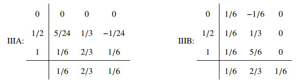
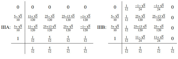
Remark 3.1. If the coefficients of a partitioned Runge-Kutta method satisfy Eq (3.2), it conserves the quadratic invariant of the form $Q(y, z) = y^{\top}Dz$ (see Ref. ^[12] for more details), thus the energy conservation law Eq (3.3) stands naturally. Moreover, the coefficients of PRK methods of order 4 and 6 are explicitly given in Tables 1 and (please see ^[20]), respectively. Hereafter, the prediction-correction scheme 3.1, coupled with 4th- and 6th-order PRK methods, are denoted by 4th- and 6th-order LEQP1, respectively. Exchanging the order of Lobatto $\rm III$ A- $\rm III$ B pairs, we further derive 4th- and 6th-order LEQP2 methods.

Table 1. Coefficients of the 3-stage Lobatto IIIA-IIIB pair.

| Show Table

DownLoad: CSV

Table 2. Coefficients of the 4-stage Lobatto IIIA-IIIB pair.

| Show Table

DownLoad: CSV

Remark 3.2. In general, a numerical algorithm, which can preserve the corresponding energy exactly, is called an energy-preserving scheme. Thus, for the semi-discrete Scheme 3.1, it should be careful to choose a suitable spatial discretization, and we need to consider the following aspects: (i) It should preserve the skew-symmetry of the operator $\mathcal D$ ; (ii) The accuracy of spatial discretization should be comparable to that of temporal counterpart. These, together with the periodic boundary condition (1.4), enlighten us to use the Fourier pseudo-spectral method for spatial discretization, which allows the application of FFT technique. In fact, the derived full discrete schemes also preserve the corresponding full discrete energy conservation law. The details are omitted here.

Remark 3.3. To our best knowledge, no theoretical result is found on the choice of iteration step $M$ . From our numerical experience, the $4th$ -order LEQP methods can reach fourth-order accuracy by choosing $M = 3$ , while the $6th$ -order LEQP methods can reach sixth-order accuracy by choosing $M = 5$ .

4. Numerical experiments

In this section, some numerical tests are carried out to investigate the accuracy, efficiency and invariants-preservation of the proposed schemes. For brevity, we only take the CH equation as a benchmark model for illustration purposes, and the corresponding prediction-correction schemes can be directly obtained by setting $\kappa = 0, \gamma = 1$ in Scheme 3.1. As shown above, the proposed scheme, which preserves the modified energy, could reach arbitrary high-order accuracy in time. Some comparisons would be made with the linearized Crank-Nicolson (IEQ-LCN) method ^[15] and energy-preserving Fourier pseudo-spectral (EPFP) method ^[9], where the wavelet collocation discretization in space is substituted by the standard Fourier pseudo-spectral method. In the following, the convergence rate in time is computed by the following formula

$\begin{align*} \quad {\rm Rate} = \frac{{\rm ln} \big(error_1/error_2)}{{\rm ln} (\tau_1/\tau_2)}, \end{align*}$

where $\tau_l, error_l \ (l = 1, 2)$ are time steps and errors with time step $\tau_l$ , respectively.

Example 4.1 We first consider the CH equation as follows

$\begin{align} \begin{aligned} & u_t-u_{xxt}+3uu_x-2u_xu_{xx}-uu_{xxx} = 0, \ (x, t) \in \Omega \times (0, T], \\ & u(x, 0) = u_0(x), \ x \in \Omega , \end{aligned} \end{align}$

(4.1)

with the following conservation laws

$\begin{align*} \mathcal M(t) = \int_{\Omega} u dx, \ \ \mathcal H(t) = -\frac{1}{2}\int_{\Omega}(u^3+uu_x^2)dx, \end{align*}$

where $u_0(x) = \text{ sin}(x), \Omega = [0, 2\pi]$ , and $\mathcal M, \mathcal H$ denote the mass and Hamiltonian energy, respectively. Moreover, the numerical "exact" solution is obtained by 6th-order LEQP1 scheme with small time step $\tau = 0.001$ and mesh size $h = 2 \pi/128$ . Numerical results involving accuracy test are shown in Table 3. As is observed that the 4th- and 6th-order LEQP methods arrive at fourth- and sixth-order convergence rates in time, respectively. What's more, they perform obviously more accurate than the other second-order schemes, while the LEQP1 schemes seem a bit more accurate than the corresponding LEQP2 schemes for both 4th- and 6th-order cases.

Table 3. Temporal errors of the numerical solutions with

$T = 1, N = 128$ .

		$\tau=1/30$	$\tau=1/60$	$\tau=1/100$	$\tau=1/120$
IEQ-LCN ^[15]	$\|\| e \|\|_{\infty, h}$	2.4481e-003	5.8420e-004	2.0830e-004	1.4438e-004
	Rate	*	2.06	2.02	2.01
	$\|\| e \|\|_h$	1.5831e-003	3.9367e-004	1.4180e-004	9.8508e-005
	Rate	*	2.01	2.00	2.00
EPFP ^[9]	$\|\| e \|\|_{\infty, h}$	4.8232e-004	1.2089e-004	4.3546e-004	3.0243e-005
	Rate	*	2.00	2.00	2.00
	$\|\| e \|\|_h$	6.1360e-004	1.5380e-004	5.5401e-005	3.8477e-005
	Rate	*	2.00	2.00	2.00
4th-order LEQP1	$\|\| e \|\|_{\infty, h}$	1.9789e-007	1.2646e-008	1.6738e-009	8.1237e-010
	Rate	*	3.97	3.96	3.96
	$\|\| e \|\|_h$	8.6448e-008	5.7624e-009	7.7034e-010	3.7448e-010
	Rate	*	3.91	3.94	3.96
4th-order LEQP2	$\|\| e \|\|_{\infty, h}$	4.8122e-007	3.1072e-008	4.0957e-009	1.9840e-009
	Rate	*	3.95	3.97	3.98
	$\|\| e \|\|_h$	2.2853e-007	1.4356e-008	1.8679e-009	9.0179e-010
	Rate	*	3.99	3.99	3.99
6th-order LEQP1	$\|\| e \|\|_{\infty, h}$	2.9625e-010	4.1179e-012	1.8738e-013	6.2783e-014
	Rate	*	6.16	6.04	6.00
	$\|\| e \|\|_h$	2.3575e-010	2.6531e-012	1.1785e-013	3.9568e-014
	Rate	*	6.47	6.09	5.99
6th-order LEQP2	$\|\| e \|\|_{\infty, h}$	8.9943e-010	1.0775e-011	4.5380e-013	1.4805e-013
	Rate	*	6.38	6.20	6.14
	$\|\| e \|\|_h$	4.9226e-010	5.0410e-012	1.9006e-013	6.0599e-014
	Rate	*	6.61	6.42	6.26

| Show Table

DownLoad: CSV

In , we show the $L^{\infty}$ -norm solution error versus the execution time for different schemes, and it can be clearly seen that the proposed high-order methods perform more effective than other second-order counterparts. Subsequently, – investigate the errors of invariants of different schemes in the long-time behaviour, where we choose $\tau = 1/3000, N = 1/128$ .

Figure 1. Comparisons of different numerical schemes.

DownLoad: Full-Size Img PowerPoint

As illustrated in Figure 1b, all schemes conserve the mass exactly. Though the proposed schemes can not preserve the exact Hamiltonian energy theoretically, the corresponding numerical errors can be preserved up to machine errors as demonstrated in Figure 1c. Moreover, Figure 1d illustrates that the proposed schemes preserve the quadratic energy precisely, which confirms the preceding theoretical analysis.

Example 4.2 In this example, we further apply the proposed method to simulate the three-peakon interaction of the CH equation with the initial condition ^[26]

$\begin{align*} u_0(x) = \phi_1(x)+\phi_2(x)+\phi_3(x), \end{align*}$

where

$\begin{align} \phi_i(x) = \left\{ \begin{aligned} & \frac{c_i}{\text{cosh}(L/2)}\text{cosh}(x-x_i), \ |x-x_i| \le L/2 , \\ & \frac{c_i}{\text{cosh}(L/2)}\text{cosh}(L-(x-x_i)), \ |x-x_i| > L/2 , \end{aligned} \right. \ i = 1, 2, 3. \end{align}$

(4.2)

The corresponding parameters are taken as $c_1 = 2, c_2 = 1, c_3 = 0.8, x_1 = -5, x_2 = -3, x_3 = -1, L = 30$ , and the computational domain is $\Omega = [0, L]$ with a periodic boundary condition.

In Figure 2a, we show the dynamics of three-peakon interaction computed by 4th-order LEQP1 scheme, and other LEQP schemes perform similarly. It is clearly seen that the moving peak interaction is resolved well. The taller wave overtakes the shorter counterparts, and afterwards they still keep their original shapes and velocities. Meanwhile, we study the invariants of the proposed schemes in long-time simulations. As demonstrated in Figures 2b–d, the proposed schemes preserve the mass and quadratic energy precisely, and perform more accurate than the IEQ-LCN method in terms of Hamiltonian energy.

Figure 2. Three-peakon simulation and comparisons of different numerical schemes.

DownLoad: Full-Size Img PowerPoint

5. Concluding remarks

In this paper, we develop a class of high-order, linearly implicit numerical algorithms, which can preserve the modified energy exactly, for the nonlinear dispersive equation. The proposed schemes, which can reach arbitrarily high-order accuracy in time, are easy to implement and computationally efficient. The key strategy lies in the application of the prediction-correction technique and the PRK method. Compared with the second-order linearly implicit structure-preserving schemes, the proposed methods perform more accurate and more efficient in longtime computations, and they can be directly applied to some relevant background problems, such as the Dai equation and regularized long wave equation in high dimensions.

Acknowledgments

Jin Cui's work is partially supported by the High Level Talents Research Foundation Project of Nanjing Vocational College of Information Technology (Grant No. YB20200906), the "Qinglan" Project of Jiangsu Province. Yayun Fu's work is partially supported by the National Natural Science Foundation of Henan Province (No. 222300420280).

Conflict of interest

The authors declare there is no conflict of interest.

References

[1]	Senneset K, Sandven R, Janbu N (1989) Evaluation of soil parameters from piezocone tests. Transp Res Rec, 24-37.
[2]	Long M, Gudjonsson G, Donohue S, et al. (2010) Engineering characterisation of Norwegian glaciomarine silt. Eng Geol 110: 51-65. doi: 10.1016/j.enggeo.2009.11.002
[3]	Blaker Ø , Carroll R, Paniagua P, et al. (2019) Halden research site: geotechnical characterization of a post glacial silt. AIMS Geosci 5: 184-234. doi: 10.3934/geosci.2019.2.184
[4]	Lunne T, Berre T, Strandvik S (1997) Sample disturbance effects in soft low plastic Norwegian clay. In: Recent Developments in Soil and Pavement Mechanics. Rio de Janeiro, Brazil: Balkema, 81-102.
[5]	Andresen A, Kolstad P (1979) The NGI 54 mm sampler for undisturbed sampling of clays and representative sampling of coarse materials. In: International Symposium on soil sampling. Singapore, 13-21.
[6]	DeJong JT, Krage CP, Albin BM, et al. (2018) Work-Based Framework for Sample Quality Evaluation of Low Plasticity Soils. J Geotech Geoenviron Eng 144: 04018074. doi: 10.1061/(ASCE)GT.1943-5606.0001941
[7]	Janbu N (1963) Soil compressibility as determined by odometer and triaxial tests. In: 3rd European Conference on Soil Mechanics and Foundation Engineering. Wiesbaden, Germany, 19-25.
[8]	Becker DE, Crooks JHA, Been K, et al. (1987) Work as a criterion for determining in situ and yield stresses in clays. Can Geotech J 24: 549-564. doi: 10.1139/t87-070
[9]	Brandon TL, Rose AT, Duncan JM (2006) Drained and Undrained Strength Interpretation for Low-Plasticity Silts. J Geotech Geoenviron Eng 132: 250-257. doi: 10.1061/(ASCE)1090-0241(2006)132:2(250)
[10]	Schneider J, Randolph M, Mayne P, et al. (2008) Analysis of Factors Influencing Soil Classification Using Normalized Piezocone Tip Resistance and Pore Pressure Parameters. J Geotech Geoenviron Eng 134: 1569-1586. doi: 10.1061/(ASCE)1090-0241(2008)134:11(1569)
[11]	Robertson P (1990) Soil classification using the cone penetration test. Can Geotech J 27: 151-158. doi: 10.1139/t90-014
[12]	Sveian H (1995) Sandsletten blir til: Stjø rdal fra fjordbunn til strandsted. Trondheim: Norges Geologiske Undersø kelse (NGU).
[13]	NGU (2020) Superficial deposits—National Database, Geological Survey of Norway (NGU). Available from: http://geo.ngu.no/kart/losmasse_mobil/?lang=eng.
[14]	Sandven R (2003) Geotechnical properties of a natural silt deposit obtained from field and laboratory tests. In: International Workshop on characterization and engineering properties of natural soils. Singapore: Balkema, 1121-1148.
[15]	Lunne T, Robertson PK, Powell JJM (1997) Cone Penetration Testing in Geotechnical Practice: Blackie Academic and Professional.
[16]	Amundsen HA, Thakur V (2018) Storage Duration Effects on Soft Clay Samples. Geotech Test J 42: 1031-1054.
[17]	NGU (2020) Arealinformasjon—Norge og Svalbard med havområ der, Geological Survey of Norway (NGU). Available from: http://geo.ngu.no/kart/arealis_mobil/?extent=296823,7044369,297380,7044631.
[18]	ISO (2012) Geotechnical investigation and testing—Field testing. Part I: Electrical cone and piezocone penetration test. Geneva, Switzerland: International Organization for Standardization (ISO).
[19]	Senneset K, Janbu N (1985) Shear strength parameters obtained from static cone penetration tests. In: ASTM Speciality Conference, Strength Testing of Marine Sediments, Laboratory and In Situ Measurements. San Diego, 41-54.
[20]	Robertson P, Campanella RG, Gillespie D, et al. (1986) Use of piezometer cone data. In: ASCE Speciality Conference In Situ '86: Use of In Situ Tests in Geotechnical Engineering. Blacksburg, 1263-1280.
[21]	Nazarian S, Stokoe KH (1984) In situ shear wave velocities from spectral analysis of surface waves. 8th World Conference on Earthquake Engineering. San Francisco, 31-38.
[22]	Park CB, Miller DM, Xia J (1999) Multichannel analysis of surface waves. Geophysics 64: 800-808. doi: 10.1190/1.1444590
[23]	Heisey JS, Stokoe KH, Meyer AH (1982) Moduli of pavement systems for spectral analysis of surface waves. In: 61^st Annual Meeting of the Transportation Research Boad. Washington, D.C., 22-31.
[24]	NIBS (2003) National Earthquake Hazard Reduction Program (NEHRP)—Recommended provisions for seismic regulations for new buildings and other structures (FEMA 450) Part 1: Provisions. Building Seismic Safety Council of the National Instiute of Building Sciences (NIBS). Washington, D.C.
[25]	Lunne T, Long M, Forsberg CF (2003) Characterization and engineering properties of Holmen, Drammen sand. Characterisation and Engineering Properties of Natural Soils. Singapore, 1121-1148.
[26]	NGF (2013) Melding 11: Veiledning for prø vetaking (in Norwegian). Oslo, Norway: Norwegian Geotechnical Society (NGF).
[27]	Terzaghi K, Peck RB, Mesri G (1996) Soil Mechanics in Engineering Practice. John Wiley and Sons.
[28]	Lunne T, Berre T, Andersen KH, et al. (2006) Effects of sample disturbance and consolidation procedures on measured shear strength of soft marine Norwegian clays. Can Geotech J 43: 726-750. doi: 10.1139/t06-040
[29]	Long M, Sandven R, Gudjonsson GT (2005) Parameterbestemmelser for siltige materialer. Delrapport C (in Norwegian). Statens Vegvesen.
[30]	Carroll R, Long M (2017) Sample Disturbance Effects in Silt. J Geotech Geoenviron Eng 143: 04017061. doi: 10.1061/(ASCE)GT.1943-5606.0001749
[31]	Donohue S, Long M (2010) Assessment of sample quality in soft clay using shear wave velocity and suction measurements. Géotechnique 60: 883-889. doi: 10.1680/geot.8.T.007.3741
[32]	Donohue S, Long M (2007) Rapid Determination of Soil Sample Quality Using Shear Wave Velocity And Suction Measurements. In: 6th International Offshore Site Investigation and Geotechnics Conference: Society for Underwater Technology, 63-72.
[33]	Krage C, Albin B, Dejong JT, et al. (2016) The Influence of In-situ Effective Stress on Sample Quality for Intermediate Soils. In: Geotechnical and Geophysical Site Characterization 5-ISC5. Gold Coast, Australia, 565-570.
[34]	Amundsen HA (2018) Storage duration effects on Norwegian low-plasticity sensitive clay samples. Trondheim: Norwegian University of Science and Technology (NTNU).
[35]	NGF (2011) Melding 2: Veiledning for symboler og definisjoner i geoteknikk—identifisering og klassifisering av jord (in Norwegian): Norwegian Geotechnical Society (NGF).
[36]	Bihs A, Nordal S, Long M, et al. (2018) Effect of piezocone penetration rate on the classification of Norwegian silt. In: Cone Penetration Testing 2018 (CPT'18), CRC Press/Balkema.
[37]	Sandbaekken G, Berre T, Lacasse S (1986) Oedometer Testing at the Norwegian Geotechnical Institute. In: Yong RN, Townsend FC, editors, Consolidation of Soils: Testing and Evaluation. West Conshohocken, PA: ASTM, 329-353.
[38]	Boone SJ (2010) A critical reappraisal of "preconsolidation pressure" interpretations using the oedometer test. Can Geotech J 47: 281-296. doi: 10.1139/T09-093
[39]	Cola S, Simonini P (2002) Mechanical behavior of silty soils of the Venice lagoon as a function of their grading characteristics. Can Geotech J 39: 879-893. doi: 10.1139/t02-037
[40]	Shipton B, Coop MR (2012) On the compression behaviour of reconstituted soils. Soils Found 52: 668-681. doi: 10.1016/j.sandf.2012.07.008
[41]	Janbu N (1985) 25^th Rankine Lecture: Soil models in offshore engineering. Géotechnique 35: 241-281. doi: 10.1680/geot.1985.35.3.241
[42]	Senneset K, Sandven R, Lunne T, et al. (1988) Piezocone tests in silty soils. ISOPT-1. Orlando: Balkema, 955-966.
[43]	Sandven R (1990) Strength and deformation properties of fine grained soils obtained from piezocone tests. Trondheim, Norway: Norwegian University of Science and Technology (NTNU).
[44]	Casagrande A (1936) The determination of pre-consolidation load and it's practical significance. In: 1^st International Soil Mechanics and Foundation Engineering Conference. Cambridge, Massachusetts, 60-64.
[45]	Grozic JLH, Lunne T, Pande S (2003) An oedometer test study on the preconsolidation stress of glaciomarine clays. Can Geotech J 40: 857-872. doi: 10.1139/t03-043
[46]	Wang JL, Vivatrat V, Rusher JR (1982) Geotechnical Properties of Alaska OCS Silts. In: Offshore Technology Conference. Houston, Texas, 20.
[47]	Berre T (1982) Triaxial Testing at the Norwegian Geotechnical Institute. Geotech Test J 5: 3-17. doi: 10.1520/GTJ10794J
[48]	Wijewickreme D, Sanin M (2006) New Sample Holder for the Preparation of Undisturbed Fine-Grained Soil Specimens for Laboratory Element Testing. Geotech Test J 29: 242-249.
[49]	Ladd CC (1991) Stability evaluation during staged construction. J Geotech Eng 117: 540-615. doi: 10.1061/(ASCE)0733-9410(1991)117:4(540)

Reader Comments

Your name:*

Email:*
© 2020 the Author(s), licensee AIMS Press. This is an open access article distributed under the terms of the Creative Commons Attribution License (http://creativecommons.org/licenses/by/4.0)