Abbreviations: CH: seismic crosshole test; CPT: cone penetration test; DPCH: direct-push crosshole test; Dr: relative density; e: void ratio; emax: maximum void ratio; emin: minimum void ratio; FC: fines content; g: acceleration due to gravity; GS: specific gravity; GWL: observed hydrostatic ground water level; IC: normalized soil behavior type index; k: hydraulic conductivity; KS: bulk modulus of soil; KW: bulk modulus of water; MW: constrained compression modulus of water; n: porosity; NZDG: New Zealand Geotechnical Database; qc: cone tip resistance; SPT: standard penetration test; TW: water temperature; USCS: Unified Soil Classification System; vp: constrained compression (P-) wave velocity; vp, w: constrained compression (P-) wave velocity of water; vs: shear (S-) wave velocity; νSK: Poisson’s ratio of the soil skeleton;
ρS: mass density of the solid soil particles; ρW: mass density of water; ωC: characteristic frequency
1.
Introduction
The evaluation of in-situ soil volumetric state (e.g., density) is fundamental to understanding the compressibility, permeability, and shear strength of soils. For engineering purposes, the volumetric state of soil is often expressed in terms of parameters such as porosity, void ratio, or relative density. These parameters are employed as a means to describe the density or compactness of the soil, and are often used directly in engineering analyses. For example, porosity is used to estimate the flow of water through soil and rock, void ratio is used in consolidation settlement analyses and critical state soil mechanics, and relative density is a key parameter in soil liquefaction analyses.
Volumetric state parameters are defined by considering that soil is a multi-phase porous material consisting of solid particles and void space, which is filled with fluid and/or gas. Soil porosity is defined as the ratio of the volume of the void space relative to the total volume of the soil (void space plus solid particles), and theoretically ranges between zero and one. Soil void ratio is defined as the volume of the void space relative to the volume of the solid particles, and theoretically ranges between zero and infinity. The porosity and void ratio may be used interchangeably and are directly related through the following equation:
While simple to define, n and e are difficult to evaluate in situ. Typically, in-situ void ratio is evaluated from high-quality, “undisturbed” soil samples collected in the field and carefully transported to the laboratory. High-quality sampling of most clayey soils is achievable and relatively inexpensive for use in geotechnical engineering practice. Hence, it is reasonable to develop good estimates of in-situ void ratio by carefully sampling the soil and performing weight-volume measurements in the lab. On the other hand, undisturbed sampling of granular materials, such as clean sands and non-plastic silts, are extremely difficult and expensive, as these soils easily densify and may completely lose their structure during sampling. Complex sampling techniques (e.g., soil freezing and gel-push sampling) can be used to obtain high-quality samples in some granular soils, but require a level of expertise and attention to detail that is beyond standard geotechnical practice. These methods are typically reserved for high-end, critical facilities or research purposes.
As sufficiently high-quality samples of granular materials are difficult to obtain, the evaluation of in-situ void ratio from laboratory measurements is rare. Given these difficulties, in-situ relative density is often estimated using empirical relationships to measurements from field penetration testing methods, such as the standard penetration test [1] and cone penetration test [2]. Kulhawy and Mayne [3] provide an overview of various Dr correlations to both uncorrected and corrected SPT N-values. The CPT has many distinct advantages over the SPT, and its popularity for geotechnical engineering purposes continues to grow [4]. Various empirical relationships have also been developed to evaluate the Dr of granular soils based on CPT measurements [3,5,6,7,8]. While these Dr empirical relationships are limited to specific soil types (e.g., quartz-based clean sands for many CPT relationships) studied in calibration chamber laboratory tests, they provide a means to estimate the compactness of soils in situ. Furthermore, if values of emin and emax for these soils are available from laboratory testing, these Dr empirical relationships may be used to estimate in-situ void ratio of granular soils. While used less frequently in geotechnical engineering, porosity relationships based on in-situ seismic wave velocity measurements have also been developed. Invasive seismic testing techniques such as crosshole (CH) seismic testing [9] are well-suited to develop high-quality measurements of constrained compression wave (i.e., P-wave) and shear wave (i.e., S-wave) propagation velocities. The use of vp and vs measurements to evaluate in-situ porosity was first considered in the petroleum industry, focusing on porous rock (e.g., sandstone) and very-dense or cemented granular soils. Wyllie et al. [10] conducted laboratory testing on various fluid-saturated, porous-media and developed the concept of a time-averaged velocity based on the vp of the solid grains (e.g., soil particles) and the vp of the fluid in the voids (e.g., water or oil). This time-averaged velocity provides a lower-limit bound on vp of the composite, porous material. As field data acquisition systems were improved and seismic testing methods were more widely adopted in practice, researchers in the 1980’s developed empirical relationships to evaluate the porosity of rock and dense granular soil based on laboratory measurements of vp and vs [11,12]. Later, empirical relationships considered the effects of clay content in the voids [13,14] and the effects of confining pressure [15]. Using the theory of linear poroelasticty [16,17] as a theoretical underpinning, coupled with the Raymer et al. [11] empirical relationship, Krief et al. [18] developed a semi-empirical relationship for porosity that better fit experimental measurements.
The theory of linear poroelasticity provides a framework to describe the propagation of small-strain stress waves through fluid-saturated, porous materials (e.g., soils) at low [16] and high [17] excitation frequencies. These materials are modeled by the superposition of the fluid and solid phases occupying the same physical space. The propagation of three different stress waves (two dilatational and one rotational) were described based on the physical properties of both the porous material and the saturating fluid. The dilatational (i.e., compression) wave of the first kind and rotational (i.e., shear) wave are P- and S-waves, respectively, commonly measured using seismic testing methods. The dilatational wave of the second kind arrives after the P-wave and is difficult to observe experimentally. Biot made the following assumptions in the development of this framework: (1) The material consists of an isotropic, linear elastic, porous solid saturated by a non-dissipative, compressible fluid. (2) The stress waves are propagated through the material in undrained conditions with no relative movement between the fluid and solid phase. Miura et al. [19] have shown this assumption is valid a low frequencies, with an upper limit at the characteristic frequency (ωC) of the soil, as defined by the following equation:
The characteristic frequency of a clean, loose sand is approximately 7 kHz, which is well above the frequencies excited during most in-situ seismic testing used for geotechnical purposes. (3) The dilatational and rotational motions induced by stress waves are uncoupled, allowing the derivation of independent wave equations describing the propagation of P- and S-waves. (4) The saturating fluid is unable to sustain shear, therefore, the small-strain shear modulus of the fluid-saturated, porous material is simply that of the porous solid.
Using Biot’s low-frequency framework, Foti et al. [20] derived a relationship that can be used to estimate soil porosity based on experimentally measured stress wave propagation velocities (i.e., vp and vs) and the physical properties of the soil, including the mass density and bulk modulus of water, the mass density and bulk modulus of the solid soil particles, and the Poisson’s ratio of the soil skeleton. By using typical values for many of the parameters, which can be reasonably assumed in most cases, the relationship may be iteratively solved to evaluate porosity using measurements of vp and vs. If the soil particles are assumed to be incompressible (i.e., KS approaches infinity), which is a reasonable assumption, then the relationship simplifies to a closed-form quadratic equation. By constraining porosity to realistic values (i.e., 0 ≤ n ≤ 1) the quadratic equation may be solved to directly evaluate porosity:
The Foti et al. [20] relationship has been used to estimate in-situ porosity (and void ratio via Eq 1) at several case history sites with mixed levels of success, as evaluated through comparisons to laboratory porosity measurements on high-quality soil samples. Foti and Lancellota [21] considered seven case histories at sites with high-quality sampling of clays. Laboratory measurements were compared to in-situ seismic-based porosity estimates from downhole testing at six of the sites and crosshole testing at the other. On average, the percent difference in porosity was less than 10% across all seven sites, with some percent differences as large as 30%. Lai and Crempien [22] numerically examined the validity of the relationship over wide ranges of vp, vs, and νSK values and found that the relationship produces non-real valued porosity estimates when vp is less than ~1450 m/s (the case when soils are not saturated). They also developed porosity estimates for a single case history site using CH testing and high-quality sampling of silty sands with moderate clay content. This porosity comparison was qualitatively described as satisfactory, however, the seismic-based estimates generally under predicted the laboratory measurements. Foti and Passeri [23] used a numerical sensitivity study to examine how errors in seismic measurements and parameter assumptions affect the porosity estimates. Errors in the measurement of vp were found to produce the largest errors in the porosity estimates. Jamilkowski [24] considered five case history sites with high-quality, undisturbed samples of a variety of soils, including clays, sands, silty sands, and mine tailings. At each of these sites, CH measurements of vp and vs were used to develop profiles of in-situ porosity. The seismic-based estimates of porosity/void ratio generally ranged from 10 to 15% different than the lab measurements, and at one clay site the seismic estimates under predicted porosity/void ratio consistently by 30 to 50%. Jamilkowski [24] concludes that in-situ evaluation of porosity via seismic measurements shows promise, but that obtaining realistic results depends on the ability to make very accurate measurements of vp and vs. He further notes that CH seismic measurements are best suited for this purpose, however, improvements are needed in order to more precisely determine wave travel time and evaluate wave travel path before seismic-based estimates of porosity/void ratio can be used in advanced geotechnical analyses.
The greatest advantages of CH testing relative to other seismic testing methods are: (1) maintaining a relatively consistent and short wave travel path, (2) preserving a strong signal-to-noise ratio as a function of depth, and (3) predominantly propagating waves through a single layer at each measurement depth. However, conventional CH testing requires drilling and casing two or three boreholes in close proximity to each other, an expense not justifiable for many geotechnical site characterization efforts. Furthermore, the soil can be disturbed significantly by drilling the boreholes and grouting the casings in place. To overcome both of these challenges, a direct-push crosshole testing method has been developed which combines the desirable aspects of CH testing (i.e., the high-quality measurements of vp and vs) with the benefits of direct-push testing methods, such as CPT [25]. DPCH testing is conducted by pushing instrumented cones into the ground using two CPT-type rigs spaced 1.5 to 2.5 m apart. Typically, seismic measurements are taken every 0.2 to 0.5 m, resulting in vp and vs profiles with high spatial resolution. The direct advancement of seismic instrumentation into the ground causes less disturbance and provides excellent coupling, ensuring the best possible measurement of seismic waves. Furthermore, the deviation/position of each instrumented cone may be tracked from depth-to-depth during testing, increasing confidence in the evaluation of the length of the wave travel path between cones. DPCH testing is significantly less expensive than traditional CH testing and is well suited for soft, near-surface (top 20 to 30 m) soils.
The use of DPCH testing accelerated greatly in the aftermath of the 2010–2011 Canterbury Earthquake Sequence, which caused unprecedented soil liquefaction damage to the city of Christchurch, New Zealand. Following these earthquakes, an extensive study was initiated to investigate the effectiveness of various shallow ground improvement methods at mitigating soil liquefaction damage to residential structures [26,27]. DPCH testing played a key role in these ground improvement trails [28,29,30,31,32] allowing for measurements of vp and vs at in the unimproved soils, in the zones of improved soil between ground improvements, and directly across ground improvement elements. Following the ground improvement trials, DPCH testing was conducted at 31 additional sites in Christchurch to contribute high-resolution profiles of vp and vs at key liquefaction/no-liquefaction case history sites [33]. Both the vp and the vs profiles played important roles in attempting to rectify a number of false-positive liquefaction case histories predicted by CPT-based simplified liquefaction triggering analyses [34]. Some of these 31 DPCH case history sites are considered herein for estimating in-situ void ratio.
The effectiveness and limitations of using high-quality in-situ measurements of vp and vs from DPCH testing to evaluate in-situ void ratio are critically examined in this paper. First, the sensitivity of the Foti et al. [20] relationship to measured and assumed input parameters (e.g., vp, vs, ρW, KW, ρS, and νSK) is evaluated through a simple parametric study applicable to soft, near-surface (top 20–30 m) soils. Then, the in-situ evaluation of void ratio of granular soils is further examined through consideration of case history sites in Christchurch, New Zealand, including ten of the 31 sites with DPCH testing mentioned above. A comparison of in-situ granular soil void ratios is developed from the following: (1) laboratory void ratio measurements on high-quality samples, (2) in-situ void ratio estimates from several CPT-based Dr empirical relationships and laboratory measurements of emin and emax, and (3) seismic-based estimates of in-situ void ratio using high-quality, high-resolution profiles of vp and vs from DPCH testing in conjunction with the Foti et al. [20] relationship.
2.
Parametric study
The Foti et al. [20] porosity relationship (see Eq 3) is a function of six parameters: vp, vs, νSK,
ρW, KW, and ρS. In soft soils, the measured vp is a function of the solid soil particle skeleton stiffness and the compressional stiffness of the pore fluid. At low degrees of saturation (e.g., less than ~98%), gas in the pore spaces limits the transmission of P-waves through the pore fluid, such that the measured vp is largely controlled by the compressional stiffness of, and the contacts between, the solid soil particles. As the soil transitions from nearly- to fully-saturated (~98% to 100%), the vp steadily increases to, and ultimately exceeds, vp of the pore fluid, which is approximately 1500 m/s for water [35,36,37]. P-wave velocities exceeding 1500 m/s are used as a screening tool to identify fully-saturated soils both in the laboratory and field. This is quite useful, as the theory of linear poroelasticity, and thus the Foti et al. [20] porosity relationship, was derived for fully-saturated soils. On the other hand, the vs of soils is only dependent on the shear stiffness of, and interactions between, the solid soil particles, because water cannot sustain shear stress. Based on a large number of DPCH case histories in the soft, near-surface soils of Christchurch, vp for fully saturated soils typically ranges from 1500 to 2000 m/s (increasing with soil skeleton compressional stiffness) and vs typically ranges from 100 to 300 m/s (also increasing with soil skeleton shear stiffness). These typical ranges are used in the void ratio parametric study developed below.
It is also important to consider typical ranges for each of the other parameters (i.e.,
νSK, ρW, KW, and ρS) and understand how assumed values may influence the evaluation of soil void ratio/porosity. The mass density and bulk modulus of fresh water are directly related to water temperature, which can easily be measured. Therefore, our void ratio sensitivity analysis will focus on only three additional parameters: (a) νSK, (b) TW, and (c) ρS. Each of these is discussed briefly below.
The Poisson’s ratio of the evacuated soil skeleton (i.e., the drained Poisson’s ratio) has been studied in the laboratory using granular soil specimens prepared and tested under varying conditions (e.g., ranges of confining pressures, relative densities, and grain size distributions). As confining pressure on the soil increases, the νSK has been shown to decrease. [38,39]. Kumar and Madhusudhan [40] found that νSK decreases with increasing relative density (i.e., decreasing void ratio). Wichtmann and Triantafyllidis [41] noted that the νSK is dependent on the grain size distribution of the soil, specifically νSK decreases as the coefficient of uniformity increases. Given the range of soils and testing conditions considered in the literature, νSK typically ranges from 0.15 to 0.35 for granular soils.
The properties of the saturating fluid (i.e., water) are represented by two parameters, the mass density and the bulk modulus. For simple purposes, typical values may be assumed for both parameters: approximately 1000 kg/m3 for ρW and 2.15 GPa for KW. However, ρW and KW are both a function of temperature and pressure [42]. The temperature of the earth is relatively stable beneath the immediate ground surface. A study considering data at 63 stations across the continental USA found that, at depths between 1 and 3 meters, the temperature of the ground typically ranges between 10 and 18 ℃ [43] During field testing, a thermometer lowered down a borehole or CPT sounding hole may be used to directly measure the ground water temperature. This is recommended to limit one source of uncertainty when estimating porosity. At atmospheric pressure, Kell [44] developed a relationship between TW and ρW. Using this relationship the ρW ranges from 999.7 to 998.6 kg/m3 (i.e., 0.1% change) over the 10–18 ℃ temperature range for near-surface soils. The effects of temperature on the compressibility of water should also be considered. The constrained-compression modulus and the bulk modulus of water are equal, because water cannot sustain shear. At small-strains, the KW may be expressed as a function of the acoustic wave (i.e., P-wave) velocity of water:
The P-wave velocity of water also varies with temperature [45]. Over the typical ground temperature range (i.e., 10–18 ℃), vp, w increases from 1447.4 m/s to 1475.9 m/s, corresponding to an increase in bulk modulus from 2.09 to 2.17 GPa (a 3.8% difference). Both the KW and ρW are directly related to the temperature of water. To simplify the parametric study, the sensitivity of void ratio estimates to KW and ρW will be considered together by changing only the single parameter, TW, over the range from 10 to 18 ℃.
The last parameter to consider is the mass density of solid soil particles, which is typically expressed relative to ρW using specific gravity. While the GS of soil particles is relatively simple to evaluate in the laboratory, it is often assumed in engineering analyses because it typically takes on a narrow range of values that is dependent on mineralogy. The GS of granular soils is typically assumed to be 2.65 (i.e., the GS of quartz/silica), but may vary between 2.6 and 2.75 depending on the specific mineralogy of the soil particles. The GS of clay minerals is higher, ranging between 2.65 and 2.85 [46]. To capture the range of GS for granular soils (e.g., sand and silts) and allow the inclusion of some clay minerals, a range of GS between 2.6 and 2.8 should be considered. Thus, if ρW is approximately 1000 kg/m3, the corresponding ρS varies between 2600 and 2800 kg/m3.
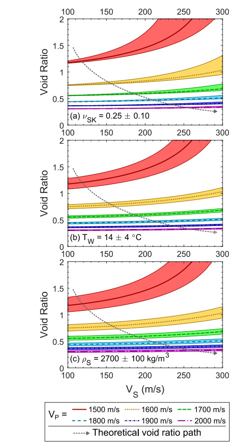
The sensitivity of the Foti et al. [20] porosity relationship to νSK, TW, and ρS is evaluated over the reasonable range of values developed above: (a) νSK = 0.25 ± 0.10, (b) TW = 14 ± 4 ℃, and (c) ρS = 2700 ± 100 kg/m3. For each analysis, one parameter is varied and the other two are held constant at the median value. Figure 1 shows the void ratio as evaluated over the typical range of S-wave velocities for soft soils (e.g., vs = 100 to 300 m/s), while P-wave velocity is held constant at one of six values ranging from 1500 to 2000 m/s, as indicated by line type. The sensitivity of the void ratio relationship to the parameter of interest (e.g., νSK in Figure 1a) is indicated by the line (i.e., the median value) and the associated shaded area (i.e., the range of values considered).
The following may be observed from Figure 1: (1) Void ratio is most strongly controlled by P-wave velocity. As vp increases, the void ratio decreases and the influence of other parameters is significantly reduced. This trend is visualized by the nearly horizontal lines and decreasing widths of the shaded void ratio ranges for vp values greater than 1700 m/s. (2) When viewed in this manner, there is an apparent contradiction with what is known to be true about the relationship between vs and void ratio: void ratio should decrease as shear stiffness increases [47,48,49,50]. Nonetheless, in Figure 1, void ratio is shown to increase as shear wave velocity increases. This seemingly contrary trend is a consequence of how the parametric study is illustrated and does not represent an error in the Foti et al. [20] relationship. In this parametric study, the void ratio is evaluated by varying vs while fixing vp. However, in real soils an increase in vs would be accompanied by a corresponding increase in vp. Hence, the void ratio path of any real soil with increasing shear stiffness would be from upper-left to lower-right in the plots of Figure 1, as indicated by the dashed arrow, and thus consistent with the literature (i.e., e decreases with increasing vs). Understanding this limitation of how the parametric study data is presented, it is still useful to note that the sensitivity of void ratio to changes in vs is severely limited as vp increases. (3) The sensitivity of void ratio to changes in νSK is dependent on vs (refer to Figure 1a). At low vs values the range of void ratios is narrow, while the range in void ratio values broadens at higher vs values. In Eq 3, the νSK term acts as a scaling factor for the square of vs, explaining this behavior. (4) While the void ratio does not appear to be overly sensitive to changes in either TW or ρS (refer to Figures 1b, c), care must be taken when assuming typical values. At vp greater than or equal to 1600 m/s, simply assuming the median water temperature (i.e., 14 ℃) yields up to an 8% error in void ratio if the in-situ TW is at the edge of the typical range. Similarly, assuming the median solid soil grain density (i.e., 2700 kg/m3) may result in an error of up to 10% if the true ρS is at the extreme of the typical range. At lower P-wave velocities, the errors in any of the other parameters may significantly change the void ratio estimate, but the magnitudes of these errors are strongly tied to vp and vs.
In summary, the Foti et al. [20] relationship for porosity based on the theory of linear poroelasticity is most sensitive to changes in vp, followed by changes in vs, νSK,
ρS, and TW (in order of decreasing sensitivity). The particular sensitivity of void ratio to vp has also been noted by Lai and Crempien [22], Jamiolkowski [24], and Foti and Passeri [23]. As suggested in the literature, typical values may be assumed for νSK, ρS, and TW (i.e., ρW and KW). However, a poor assumption (even within the range of typical values) for any parameter may produce errors as large as 10% in void ratio, underscoring the importance of using site and soil specific values whenever possible (e.g., measure the ground water temperature and evaluate the specific gravity of the soil).
3.
Datasets
Ideally, the seismic-based estimates of in-situ void ratio from DPCH testing should be directly compared to void ratio measurements from laboratory testing on high-quality granular soil samples. At seven sites with DPCH testing in Christchurch, several high-quality samples of predominantly silty soils (e.g., silts, sandy silts, and silty sands) were collected to study their cyclic stress-strain behavior [51,52]. However, most of the corresponding DPCH measurements at these sites indicate that these silty soils were not fully saturated in situ (i.e., vp < 1500 m/s). Hence, the Foti et al. [20] porosity relationship could not be used at these sites. Many of the DPCH datasets in Christchurch indicate that sandy soils typically do not become fully saturated for 1–2 m below the GWL. This unsaturated transition zone is even more significant for silty soils, with some silty soils not reaching full saturation for 5–6 m below the GWL. Since fully saturated conditions are needed to estimate void ratio, predominantly sandy soil sites are the focus of this study.
Ten predominantly sand (e.g., clean sand and silty sand) case history sites with both DPCH and CPT testing were identified from the 31 DPCH case history sites in Christchurch. However, high-quality granular soil samples were not collected at any of these sites. So, seismic-based estimates of void ratio at these ten DPCH sites cannot be directly compared to those obtained from high-quality samples. Nonetheless, high-quality samples of sand obtained from gel-push sampling were available in the same geologic formations at two other sites in Christchurch [53]. As CPT soundings are available for both sets of case histories, an examination of the effectiveness of using DPCH seismic-measurements to estimate in-situ void ratio is developed below in two parts: (1) The laboratory measurements of void ratio on high-quality gel-push specimens at two sites, including statistical ranges for emin and emax, are used to “calibrate” the CPT-based estimates of void ratio. (2) Using insight gained from this comparison, the CPT-based estimates of in-situ void ratio are directly compared to the seismic-based estimates of void ratio at the ten predominantly sand DPCH case history sites.
3.1. Sites with high-quality soil sampling of sands and silty sands
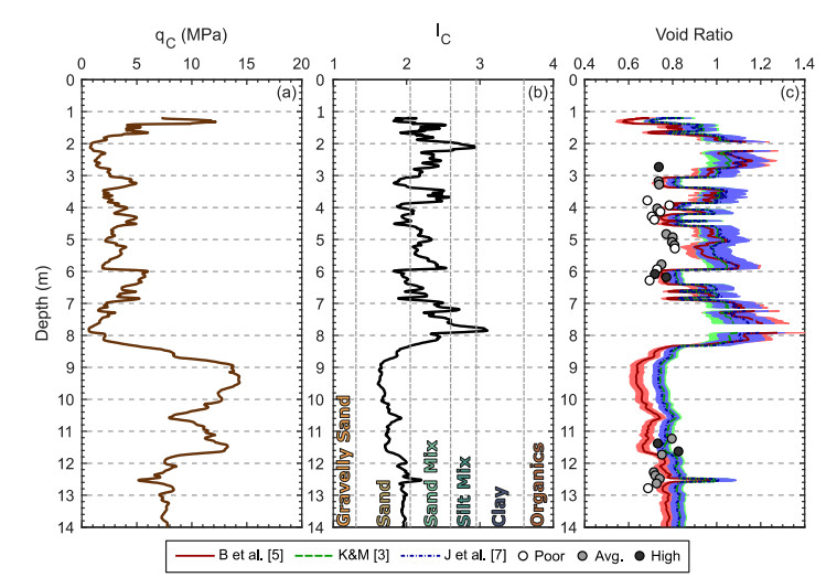
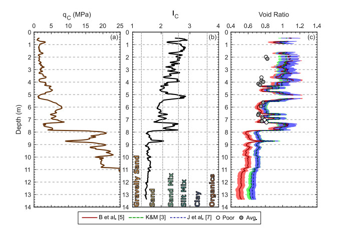
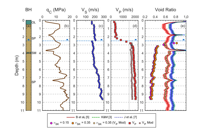
At two sites located in the central business district of Christchurch, several high-quality sand samples were collected using a gel-push sampler in an effort to characterize the behavior of typical Christchurch sandy soils under cyclic loading conditions [53]. These sites were targeted due to the manifestation of liquefaction following the 2010–2011 Canterbury Earthquake Sequence and availability of CPT data nearby [54]. Figures 2 and 3 show the: (a) cone tip resistance and (b) normalized soil behavior type index from CPT soundings located at the Kilmore Street and Madras-Armagh sites, respectively. The near-surface soil profile at the Kilmore St. site consists of a 2-m thick man-made gravel layer, a 6-m thick layer of silty sand of the Springston Formation, and a clean medium-grained sand layer of the Christchurch Formation. The gel-push sampling targeted both the silty sand and clean sand layers (Figure 2c). The silty sand samples from the Springston Formation, obtained at depths between 2.5–6.5 m, had fines contents ranging from 20% to 50%, while the clean sands from the Christchurch Formation had FC ≤ 5%, based on sampling between 11 and 13 m. At the Madras-Armagh site, the silty sand of the Springston Formation (20% ≤ FC ≤ 50%) was again targeted for sampling at 2 m, 3.5 to 4.5 m, and 5.5 to 7 m, as indicated in Figure 3c. The suite of laboratory tests on specimens obtained via gel-push sampling included measurement of, presumably, in-situ void ratio as individual specimens were consolidated and prepared for subsequent monotonic- and cyclic-strength testing, and the evaluation of emin and emax on reconstituted specimens. In Figures 2c and 3c, the laboratory void ratio measurements, indicated by circular markers, are compared with CPT-based estimates of in-situ void ratio.
CPT measurements are typically correlated to relative density, rather than directly to void ratio or porosity. These empirical relationships have been developed primarily from laboratory calibration chamber testing on various clean sands. Thus, the CPT-based relationships for Dr are less reliable when applied to soils with increasing FC. In this study, three CPT-based relative density empirical relationships are considered: Baldi et al. [5], Kulhawy and Mayne [3], and Jamiolkowski et al. [7]. Thus, three Dr estimates are obtained for each CPT measurement. Using these Dr estimates and appropriate values of emin and emax, in-situ void ratio can be evaluated using the following equation:
The laboratory characterization of both emin and emax are inherently difficult and subjective. Rather than develop single representative values of emin or emax, reasonable ranges have been developed from the Taylor [53] dataset. The soils and associated testing results were bundled into two groups: (1) clean sands of the Christchurch Formation from the Kilmore St. site and (2) silty sands of the Springston Formation, including samples from both sites. The laboratory measurements of emin and emax were separated by group and assumed to be normally distributed to develop representative mean and standard deviation values (summarized in Table 1). As fines content measurements are not always available, these emin and emax values are assigned to each individual CPT measurement based on the IC values, as follows: (1) If IC is less than 2.05, the clean sand emin and emax values are assigned. (2) If IC ranges between 2.05 and 2.60, the silty sand emin and emax values are assigned. (3) If IC exceeds 2.6, the soil is considered predominantly fine-grained (silty), the associated CPT-based Dr estimates are unreasonable, and emin and emax values are not assigned.
The uncertainties associated with emin and emax also need to be addressed in the estimation of void ratio. The relative contribution of uncertainty to the void ratio estimates from either emin or emax changes with Dr, according to Eq 5. For example, as Dr increases, the uncertainty contribution from emin increases and the uncertainty contribution from emax is diminished. Thus, the uncertainty in an individual CPT-based void ratio estimate needs to consider the relative uncertainty contribution from both emin and emax as a function of each individual Dr estimate. In order to account for this, a series of Monte Carlo simulations was used to develop 100,000 different realizations of void ratio for each individual Dr estimate. For each realization, independent random values of emin and emax are generated based on the associated mean and standard deviation values (refer to Table 1) for the appropriate soil type. As emin and emax are both assumed to be normally distributed, the associated void ratio estimate will also be normally distributed, following the Central Limit Theorem. The mean and standard deviation of the 100,000 void ratio realizations are then used to establish the mean and the ±1 standard deviation bounds for each individual CPT-based estimate of in-situ void ratio.
The CPT-based in-situ void ratio estimates developed from three Dr empirical relationships (Baldi et al. [5], Kulhawy and Mayne [3], and Jamiolkowski et al. [7]) and soil-type specific emin and emax values are shown in Figures 2c and 3c. The associated mean in-situ void ratio estimates are indicated by solid, dashed, and dot-dashed lines for each CPT- Dr relationship, respectively. The ±1 standard deviation bounds for the void ratio estimates are indicated by the shaded areas. The Baldi et al. [5] relationship consistently yields lower void ratio estimates compared to the other two relationships, which provide similar estimates of void ratio over the range of soil types. Specifically, in clean sands (e.g., below 8.5 m in Figure 2c and below 8 m in Figure 3c) the Baldi et al. [5] void ratio estimates are on average 15% lower, and as qc increases the estimates separate further. These CPT-based void ratio estimates are directly compared with the laboratory void ratio measurements from gel-push samples, which are indicated by circular markers in Figures 2c and 3c; the relative sample quality descriptions provided by Taylor [53] (i.e., poor, average, or high) are indicated by the circular marker fill.
First, consider the clean sand samples from Kilmore St., which occur at depths between 11–13 m (see Figure 2c). The CPT-based estimates of in-situ void ratio compare favorably with the laboratory values. This is expected as the CPT-based Dr empirical relationships were developed based on laboratory testing in clean sands. In contrast, the in-situ void ratios of the silty sands, sampled at depths between 2.5 and 6.5 meters, were estimated with mixed levels of success. The measured fines contents in these soil specimens were quite variable, generally ranging between 20% and 50%. However, a few of these specimens had fines contents as high as 80%. This fines content variability is reflected in qc, IC, and the resulting void ratio estimates. In general, the CPT-based void ratio estimates are greater than the measured values in the silty sands, especially estimates based on lower qc values. Given that many of these specimens were also of average to poor quality, it is hard to say if the CPT estimates are “wrong” or if the specimen measurements are “wrong”. More than likely it is a combination of both factors.
Additional comparisons of measured and estimated void ratio for the silty sand at the Madras-Armagh site are shown in Figure 3c. These samples are, in general, higher quality than those obtained in the silty sand at Kilmore St. At this site, the silty sands can be separated into two distinct groups based on cone tip resistance. Above 5.5 m, the qc is less than 5 MPa and the corresponding CPT-based void ratio estimates are consistently greater than the laboratory measurements. On the other hand, when qc exceeds 5 MPa, the associated IC values are below 2.05 (indicating a sand normalized soil behavior type) and the measured and estimated void ratios agree quite well.
In summary, this dataset provides valuable insight into the performance of CPT-based relative density relationships in sandy soils of the Springston and Christchurch Formations. The CPT-based estimates of void ratio are best in sands with relatively low fines contents, when IC is less than 2.05 and qc is greater than about 5MPa. The CPT-based estimates apparently over estimate void ratio for silty sands with higher fines content, when IC exceeds 2.05 and qc is less than 5 MPa. This qualitative calibration of the CPT-based Dr relationships for the sandy-soils (e.g., clean sands and silty sands) in Christchurch, coupled with the representative emin and emax ranges, allows meaningful comparisons of CPT-based empirical estimates of void ratio with those obtained from DPCH seismic measurements at other sites in Christchurch with similar soils.
3.2. Sand sites with DPCH testing
As noted above, ten sites with DPCH measurements of vp and vs were selected for seismic-based estimation of in-situ void ratio based on the following criteria: (1) the sonic borehole logs, IC profiles, and geology indicated that the soils were predominately sandy and similar to those studied in the Taylor [53] case histories, (2) the DPCH data was of the highest quality, with the best possible cone deviation and waveform measurements, and (3) the sandy-soils were saturated over most of the depth range, as indicated by vp measurements greater than 1500 m/s. It should be noted that soil profiles at these ten sites predominately consist of sandy soils (e.g., clean sands and silty sands), however, silty soil (e.g., silt and sandy silt) deposits, with appreciable fines contents (FC > 20%), may also be present. On a case-by-case basis, individual silty soil deposits may be included in the comparison below, depending on measured IC and qc, as discussed above. The geotechnical site investigation data (e.g., sonic borehole log, CPT sounding, and DPCH vp & vs profiles) at each of these sites may be found in the New Zealand Geotechnical Database (https://www.nzgd.org.nz). The ten site names and NZGD DPCH testing reference numbers are summarized in Table 2. The CPT and DPCH measurements have been used in the development and comparison of in-situ void ratio estimates, as described below.
The Baldi et al. [5], Kulhawy and Mayne [3], and Jamiolkowski et al. [7] CPT-based Dr empirical relationships have been used to estimate in-situ void ratios at each of the ten sites. The CPT-based estimates of void ratio are compared with those obtained from the DPCH vp and vs measurements using the Foti et al. [20] porosity relationship developed from the theory of linear poroelasticity. As noted in the parametric study, this relationship requires the evaluation or assumption of several other parameters (i.e., νSK, ρW, KW, and ρS). After vp and vs, the void ratio is most sensitive to νSK. Hence, in order to account for uncertainty, the seismic-based void ratio estimates are evaluated at νSK equal to 0.15 and 0.35, capturing the typical range of values. The density and bulk modulus of water have been shown to vary with water temperature. The temperature of the ground water is assumed to be 14 ℃, the median of near-surface ground temperatures discussed above. Given laboratory testing results on similar soils from the Taylor [53] study, the density of the solid soil grains is assumed to be 2700 kg/m3.
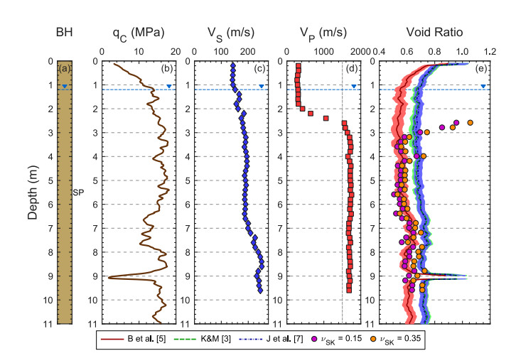
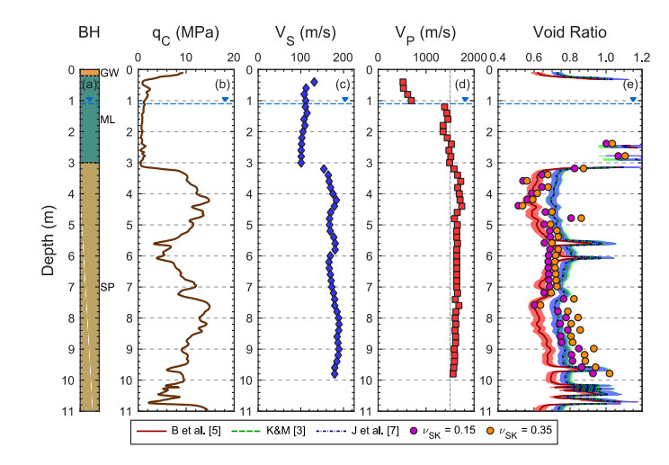
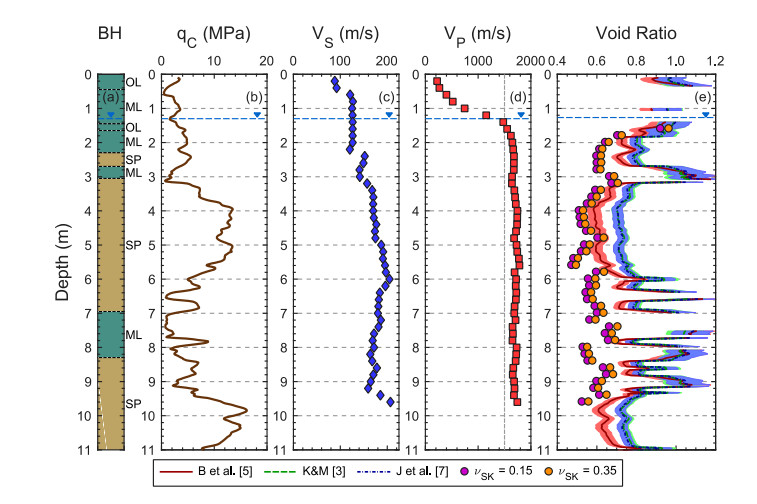
To highlight the varying levels of agreement between the CPT-based and seismic-based void ratio estimates, four of the ten sites are discussed in detail below: (1) Rawhiti Domain, (2) Charles Street, (3) Palinurus Road, and (4) Carisbrooke Playground. Figures 4 through 7 present the void ratio estimates and supporting geotechnical data at each of these sites in a five-panel format: (a) sonic borehole log with USCS soil classifications, (b) qc, (c) vs, (d) vp, and (e) void ratio estimates.
The Rawhiti Reserve dataset (see Figure 4) represents the highest level of agreement between the seismic- and CPT-based in-situ void ratio estimates of our ten case history sites. The near-surface soil profile is solely comprised of clean sands of the Christchurch Formation. Limited specimens tested from disturbed sonic sampling at this site indicate fines contents lower than 5%. The qc values generally range between 10–20 MPa, while the vs values range from about 140–240 m/s. Even though the GWL is located just below 1 m, the vp values do not indicate that the soil is saturated until near 2.5 m. Below 3 m, the seismic-based void ratio estimates agree well with the CPT-based Baldi et al. [5] estimates, with void ratios calculated from both νSK values falling in or near the ±1σ bounds of the CPT relationship. A few important observations should be highlighted: (1) As noted in the parametric study (refer to Figure 1), the Foti et al. [20] relationship is very sensitive to slight changes in vp. The void ratio estimates are unstable from 2.6 to 3 meters as the soil is just reaching full saturation and vp increases from 1500 to 1700 m/s. At 4 meters, a small (3%) decrease in vp results in a 12% jump in the void ratio estimate. (2) The seismic-based estimates are relatively insensitive to the assumed νSK value until vs exceeds about 200 m/s at depths greater than 7 m. This effect was also noted in the parametric study (refer to Figure 1a). (3) In general, there is excellent agreement between in-situ void ratio estimates developed from DPCH measurements and the Baldi et al. [5] CPT relationship. When differences do exist, it is impossible to say which method is “better”, particularly since fairly significant differences in-void ratio exist between Baldi et al. [5] and the other two CPT-based relationships.
The Charles Street dataset, as shown in Figure 5, illustrates the impact of increased fines content and reflects greater disagreements in the void ratio estimates. A 3-m thick deposit of low plasticity silt of the Springston Formation overlies clean sands of the Christchurch Formation. The silt-to-sand transition is marked by a sharp increase in soil stiffness, as indicated by an increase in qc from 0.5 to 10 MPa and a jump in vs from 100 to 155 m/s. The observed GWL at 1.1 m is marked by a sharp increase vp from 700 to 1350 m/s. The soil remains nearly saturated in the silt layer. At the silt-to-sand transition, vp increases to 1600 m/s, reflecting both the increase in soil skeleton stiffness and full saturation of the soil. In the silty-soil deposit, high fines contents and IC greater than 2.6 prohibit reasonable evaluation of the CPT-based void ratio, except at two localized measurement depths, 2.4 and 2.8 m, where IC < 2.6. The seismic-based void ratio estimates at these two depths fall within the ±1σ bounds of the CPT-based estimates, showing a high-level of agreement despite the silty soil conditions. The void ratio comparisons in the clean sand should be considered in three distinct depth ranges: (1) 3.2 to 5 m, (2) 5 to 7.2 m, and (3) 7.4 to 9.8 m. From 3.2 to 5 m, the measured vp reaches 1750 m/s as the qc approaches 15 MPa. The associated seismic-based void ratio estimates agree best with the Baldi et al. [5] estimates over most of this range. At measurement depths between 5 and 7.2 m, the vp profile stabilizes at ~1650 m/s, resulting in consistent void ratio estimates of approximately 0.65 to 0.73, depending on νSK. The associated CPT-based estimates of void ratio gradually change with qc, however, the seismic-based estimates generally fall within the Baldi et al. [5] bounds. Below 7.4 meters, the qc values gradually decrease and similar trends are observed in the vp and vs profiles. Specifically, vp decreases from about 1650 to 1550 m/s, corresponding to an increase in void ratio of about 0.30 (from about 0.7 to about 1.0). Over the same depth range, each of the three CPT-based estimates increase by only 0.05. The void ratio estimates over all three depth ranges underscore the sensitivity of the seismic-based void ratios to changes in vp. While there is remarkable agreement in the trends between qc and vp, it appears that the seismic-based void ratio estimates below 7.4 meters may be changing too much because the seismic void ratio estimates are very sensitive when vp is near 1500 m/s.
The Palinurus Road dataset (see Figure 6) highlights disagreement between seismic- and CPT-based void ratio estimates in soils with increased fines content. At this site, a 3-m thick deposit of silts and silty sands of the Springston Formation overlies clean sands of the Christchurch Formation. The transitions between these soils are clearly reflected in qc, which exceeds 10 MPa in the clean sands and is lower than 3 MPa in the silty sands and silts. In the clean sands, the seismic-based void ratios are slightly lower than the Baldi et al. [5] −1σ bound. Given better agreement in clean sands at the two previously discussed sites, low seismic void ratio estimates at this site may indicate slightly high/inaccurate vp measurements at this site. The seismic-based void ratio estimates in the silty sands are substantially lower than those obtained from the CPT relationships over the depth range of 6.0–9.5 m. As noted above, the CPT-based estimates are not very reliable in silty sands, and likely too high. While the Foti et al. [20] porosity relationship should be valid for these silty sands, the void ratio estimates from seismic DPCH testing are suspected to be too low, and likely caused by slightly high vp values. However, the seismic-based void ratio estimates cannot be quantitatively evaluated in the silty sands given the limitations of the CPT-based relationships.
The last of the four selected sites, Carisbrooke Playground (see Figure 7), represents the greatest level of disagreement between seismic- and CPT-based estimates of void ratio at all ten sites considered. Here, a thin, silt surface layer overlies a thick deposit of clean sands of the Christchurch Formation. Generally, the stiffness of the clean sands steadily increases below the observed GWL, as indicated by several measurements: qc increases from 10 to 18 MPa, vs increases from 170 to 270 m/s, and vp increases from 1650 to 2050 m/s. While vp is high, the relatively high qc and vs lend some confidence to these measurements. Given the predominantly clean sand profile, a high level of agreement between the seismic- and CPT-based estimates of void ratio is anticipated. However, the seismic-based estimates range between 0.33 and 0.45, significantly lower than those developed from any of the three CPT-based Dr empirical relationships and lower than one would expect (significantly lower than the emin values indicated in Table 1). Even relative to the lowest CPT-based estimates of Baldi et al. [5], the seismic-based estimates are 55 to 70% lower.
Given the better agreement between seismic- and CPT-based estimates of in-situ void ratio at the other example sties, it is important to investigate potential causes for this disagreement. At the Carisbrooke Playground, vp measurements exceed 1800 m/s in the fully-saturated soils. According to the results of the sensitivity study shown in Figure 1, these high P-wave velocities essentially limit the effect that vs (or any other parameter) has on the void ratio. Specifically, when vp is equal to 1800 m/s the seismic-based void ratio estimates are restricted to values of about 0.4–0.5, irrespective of vs changing over 200% from 100 to 300 m/s. So, it is clear that the high vp values at this site are governing the apparently low seismic-based estimates of void ratio. Assuming the mean Baldi et al.
[5] void ratio profile reasonably reflects the in-situ conditions, and νSK is equal to 0.35, the percent decrease in vp required to make the seismic- and CPT-based void ratios match was investigated. It was determined that the original vp measurements (ranging from 1700 to 2050 m/s) only needed to be reduced by 9 to 16% percent (refer to the vp Mod symbols in Figure 7d) in order to match the Baldi et al. [5] void ratio estimates (refer to the νSK = 0.35 (vp Mod symbols) in Figure 7e). The modified vp profile ranges from 1625 to 1775 m/s. A slightly, larger reduction (up to 18%) in vp is necessary to match the other CPT relationships.
4.
Discussion
Given that seismic-based void ratio estimates are so sensitive to vp measurements, it is important to consider the accuracy of vp (and vs) obtained from DPCH testing. Seismic waves are assumed to directly travel along a horizontal path from the source to the receiver. At each measurement depth, the seismic wave velocities (i.e. distance per unit time) are evaluated by dividing the length of the travel path by the associated wave travel time. Measurement errors in travel path length and/or time are carried into the velocity evaluation. In the fully-saturated Christchurch sands, vp generally ranges from 1500 to 1850 m/s and vs generally ranges from 80 to 250 m/s, depending on the density, state of stress, and soil skeleton stiffness. Assuming the P- and S-waves travel along the same travel path from source to receiver, a 10% measurement error in the travel path length results in a 10% error in both vp and vs. However, in fully-saturated soils the P-wave travel time is an order of magnitude smaller than the S-wave travel time. A 10% error in the travel path may change the vs by 8 to 30 m/s, while the corresponding vp may be off by 150 to 185 m/s. As noted in the parametric study, the void ratio estimates would minimally change due to this error in vs (see Figure 1), but would be greatly altered by the corresponding error in vp. At the Carrisbrooke Playground and Charles Street sites, the vp profiles appear to gradually drift. In part, this may be due to the gradual changes in the stiffness of the soil skeleton, as observed in qc. However, this drift may also reflect a systematic, cumulative error in determining the travel path distance. In DPCH testing, the distance between the cones is evaluated based on the cone positions, which are updated based on changes in the tilt angles and push distance between each seismic measurement depth. Thus any measurement errors are carried through each successive testing depth. Another potential source of error in vp (and vs) is the evaluation of the direct wave travel times. As noted in Cox et al. [25], timing errors in DPCH testing may arise from several sources: the misidentification of the direct arrivals, improper consideration/calibration of data acquisition triggering, and noise in the recorded waveforms. While P-wave arrivals in saturated soils are high-frequency and relatively easy to identify, noise and poor triggering may obscure the arrival. At typical sampling rates (~20 kHz) and travel path lengths (1 to 3 m, depending on cone deviation), picking a trigger time or wave arrival time that is in error by only a single time sample may result in a vp error as large as ~5%. As the waveforms are independently generated and measured at each testing depth, the minor timing errors are likely isolated to individual or small subsets of velocity measurements. For example, the slightly decreased vp at a depth of 4 meters at the Rawhiti Reserve (see Figure 4) may be caused by such a timing error.
Given that undisturbed soil samples have not been obtained at the case history sites where high-resolution DPCH vp and vs data are available, it is impossible to know what the “true” void ratios at these sites are. However, across all ten of the predominantly sand sites discussed in this paper, the following trends have been observed: (1) the CPT-based void ratio estimates vary from one another, with those from Baldi et al. [5] being on average 10–15% less than the others, (2) the seismic-based void ratio estimates tend to agree best with the CPT-based estimates of Baldi et al. [5], and (3) in some cases it appears that the seismic-based void ratio estimates may be too low due to suspected small errors in measuring vp (potentially caused by errors in the tilt/distance calculations). The impact of potential small errors in vp is investigated further by considering the percent change in vp needed in order to make the seismic-based void ratio estimates match those of the CPT-based estimates. This exercise is similar to what was performed above at the Carrisbrooke Playground site. However, it is now expanded to consider the nine other sand sites in our database. Note that the Carrisbrooke Playground site is not considered further below since the seismic-based void ratio estimates have already been shown to be suspiciously low and likely in error.
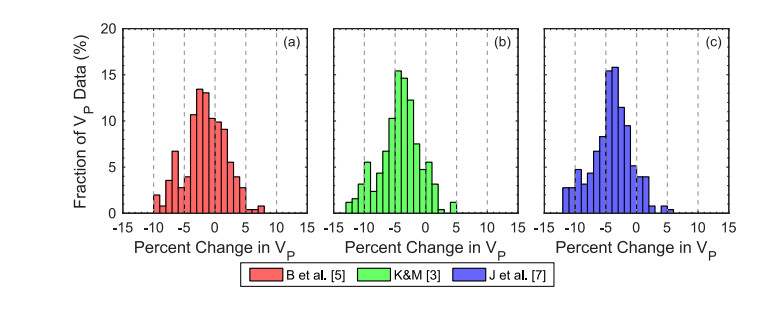
Neglecting measurements made in silty sands with IC greater than 2.05,253 distinct vp and vs seismic measurements were made in soils consisting of clean sands, across nine sites. The void ratio estimates from these 253 seismic measurements have been statistically compared to the median values of the CPT-based void ratio estimates by computing the percent change in vp required to bring these estimates into agreement with one another. To simplify these comparisons, the seismic-based void ratio estimates were evaluated using a single νSK value of 0.25. In Figure 8, the distributions of required percent changes in vp are presented in three histograms, one for each CPT relationship: (a) Baldi et al. [5], (b) Kulhawy and Mayne [3], and (c) Jamiolkowski et al. [7]. The width of each histogram bin represents a 1% change in vp. Each of these histograms are approximately bell-shaped. The peak of the bell is centered at approximately −2%, −4%, and −4% change in vp for the Baldi et al. [5], Kulhawy and Mayne [3], and Jamiolkowski et al.
[7] relationships, respectively. Meaning, on average, only a slight decrease in vp is needed to bring the seismic-based void ratio estimates into agreement with the CPT-based estimates. These small changes in vp are within the range of potential measurement errors in DPCH testing. Hence, improvements need to be made to seismic testing methods such that vp can be evaluated within 1–2% in order to have confidence in the seismic-based void ratio estimates.
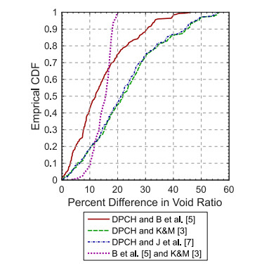
It is also important to quantify the difference between seismic-based and CPT-based void ratio estimates beyond qualitative observations. To this end, the percent difference between the seismic-based void ratio estimates (with νSK = 0.25) and each of the three CPT-based estimates were evaluated for the 253 clean sand data points. In addition, the percent difference between the Baldi et al. [5] and the Kulhawy and Mayne [3] CPT-based void ratio estimates was also evaluated for the same 253 clean sand data points. The empirical cumulative distribution functions for each set of percent differences in estimated void ratio are shown together in Figure 9. First, consider the percentage of DPCH seismic-based void ratio estimates that are within 10% of the CPT-based estimates: approximately 43% relative to Baldi et al. [5] and approximately 19% relative to the other two CPT relationships. While these numbers may not seem great, it should be noted that only about 9% of the void ratio estimates of Baldi et al. [5] and Kulhawy and Mayne [3] agree within 10% of one another. In fact, for more than 65% of the data points considered, the Baldi et al. [5] CPT-based estimates agree better with the seismic-based estimates than with the other CPT-based estimates. However, for the remaining 35% of the data points, the maximum percent difference between the CPT-based estimates is no more than 20%, while the maximum percent difference between the seismic- and CPT-based estimates ranges from about 45% to 55%. These large differences are most likely attributed to small errors in determining vp, which typically result in the underestimation of void ratio. Statistically, the DPCH vp and vs measurements coupled with the Foti et al. [20] theoretical relationship proved to be relatively effective at evaluating the in-situ void ratio of clean sands when compared to the CPT-based relationships.
5.
Conclusion
A relationship to evaluate soil porosity (i.e., void ratio) in fully-saturated soils from seismic wave propagation velocities (i.e., vp and vs) was developed by Foti et al. [20] using the theory of linear poroelasticity [16,17] as an underlying framework. Soil porosity is evaluated as a function of vp, vs and four additional parameters describing the physical properties of the soil (i.e., νSK, ρS, ρW, and KW). In this study, the effectiveness and feasibility of using high-resolution vp and vs measurements from DPCH testing to estimate in-situ void ratios was investigated at ten, predominantly clean sand case history sites in Christchurch, New Zealand. As high-quality, “undisturbed” samples were not available at these ten sites, absolute comparisons of in-situ void ratio estimates could not be made. Hence, only relative comparisons could be made between CPT-based estimates of in-situ void ratio and those obtained from seismic measurements. Nonetheless, the CPT-based estimates of in-situ void ratio were “calibrated” using soil-specific emin and emax values, including associated uncertainties, and were demonstrated to yield fairly consistent agreement with void ratio measurements obtained from gel-push samples of sand at two other sites in Christchurch.
Detailed comparisons between seismic- and CPT-based void ratio estimates have been shown at four sites, where agreement between estimates ranges from excellent to poor. From a statistical analysis of 253 seismic-based void ratio estimates across nine of the ten sites considered in this study, it was found that approximately 43% of the in-situ void ratio estimates for the clean sand data points fell within 10% of the Baldi et al. [5] CPT-based estimates. While this agreement may not seem amazing, it should be noted that only about 9% of the CPT-based void ratio estimates of Baldi et al. [5] agree within 10% of the CPT-based estimates of Kulhawy and Mayne [3] and Jamiolkowski et al. [7]. In fact, for more than 65% of the data points considered, the Baldi et al. [5] CPT-based estimates agree better with the seismic-based estimates than with the other CPT-based estimates. However, for the remaining 35% of the data points, the maximum percent difference between the CPT-based void ratios is no more than 20%, while the maximum percent difference between the seismic- and CPT-based void ratios ranges from about 45% to 55%. These large differences are attributed to small errors in determining vp, which result in significant underestimation of void ratio. While the “true” void ratios in this study are not known, when very poor agreement between seismic- and CPT-based estimates of void ratio are observed in clean sands, the authors believe the seismic-based estimates are most likely in error. However, it has been demonstrated that only moderate adjustments to vp (2 to 4% on average) are required to bring the seismic- and CPT-based void ratio estimates into agreement with one another. This finding is both encouraging and discouraging; encouraging because estimating void ratio based on in-situ measurements of vp and vs seems attainable, and discouraging because it is extremely difficult to measure any parameter in situ within 2%.
We believe that DPCH testing has the potential to enable very high-resolution measurements of vp and vs. With slight improvements to the equipment and testing procedures we hope to be able to track cone deviations and resolve P-wave travels times even more accurately. If this can be done, more consistent and reliable estimates of in-situ void ratio can be obtained from linear poroelasticity theory, which is valid for all fluid-saturated porous materials (e.g., sands, silts, and clays). Estimating void ratio in this way is much more satisfying than continuing to rely on empirical correlations to penetration resistance that also show significant scatter and, at best, are currently only appropriate for use in clean sands. Additional case histories are needed to increase confidence in void ratio estimates made via DPCH seismic measurements through direct comparisons with laboratory measured void ratios on high-quality samples of both granular and cohesive soils.
Acknowledgments
This work was partially supported by U.S. National Science Foundation (NSF) grant CMMI-1547777, the N.Z. Earthquake Commission (EQC), QuakeCoRE, and the University of Canterbury. However, any opinions, findings, conclusions, or recommendations expressed in this material are those of the authors and do not necessarily reflect the views of the sponsors. We would also like to thank and acknowledge Dr.’s Sjoerd van Ballegooy and Liam Wotherspoon for their help in coordinating and aiding the field data collection of DPCH measurements at these case history sites. Additionally, this article was strengthened by peer-review comments from several referees. We would like to thank them for their contributions.
Conflict of interest
All authors declare no conflicts of interest in this paper.


 DownLoad: