Aspects of activation, selection and control have been related to attention from early to more recent theoretical models. In this review paper, we present information about different levels of analysis of all three aspects involved in this central function of cognition. Studies in the field of Cognitive Psychology have provided information about the cognitive operations associated with each function as well as experimental tasks to measure them. Using these methods, neuroimaging studies have revealed the circuitry and chronometry of brain reactions while individuals perform marker tasks, aside from neuromodulators involved in each network. Information on the anatomy and circuitry of attention is key to research approaching the neural mechanisms involved in individual differences in efficiency, and how they relate to maturational and genetic/environmental influences. Also, understanding the neural mechanisms related to attention networks provides a way to examine the impact of interventions designed to improve attention skills. In the last section of the paper, we emphasize the importance of the neuroscience approach in order to connect cognition and behavior to underpinning biological and molecular mechanisms providing a framework that is informative to many central aspects of cognition, such as development, psychopathology and intervention.
Citation: M. Rosario Rueda, Joan P. Pozuelos, Lina M. Cómbita, Lina M. Cómbita. Cognitive Neuroscience of Attention From brain mechanisms to individual differences in efficiency[J]. AIMS Neuroscience, 2015, 2(4): 183-202. doi: 10.3934/Neuroscience.2015.4.183
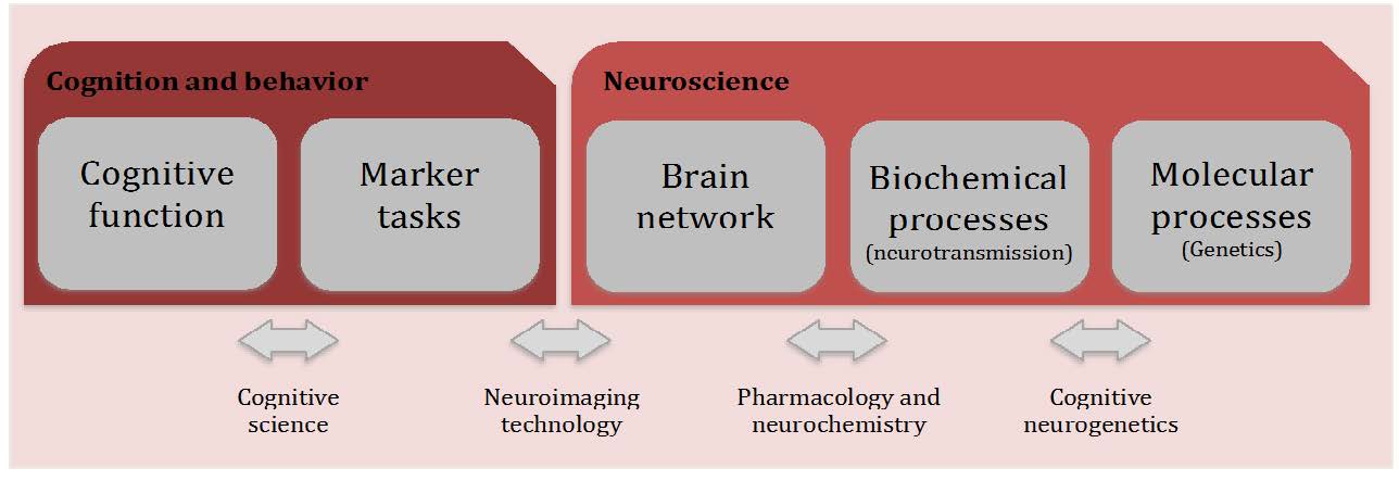
Aspects of activation, selection and control have been related to attention from early to more recent theoretical models. In this review paper, we present information about different levels of analysis of all three aspects involved in this central function of cognition. Studies in the field of Cognitive Psychology have provided information about the cognitive operations associated with each function as well as experimental tasks to measure them. Using these methods, neuroimaging studies have revealed the circuitry and chronometry of brain reactions while individuals perform marker tasks, aside from neuromodulators involved in each network. Information on the anatomy and circuitry of attention is key to research approaching the neural mechanisms involved in individual differences in efficiency, and how they relate to maturational and genetic/environmental influences. Also, understanding the neural mechanisms related to attention networks provides a way to examine the impact of interventions designed to improve attention skills. In the last section of the paper, we emphasize the importance of the neuroscience approach in order to connect cognition and behavior to underpinning biological and molecular mechanisms providing a framework that is informative to many central aspects of cognition, such as development, psychopathology and intervention.

| [1] | James W (1890) The principles of psychology (H. Holt, New York, NY). |
| [2] |
Posner MI, Petersen SE (1990) The attention system of the human brain. Annu Rev Neurosci 13: 25-42. doi: 10.1146/annurev.ne.13.030190.000325

|
| [3] | Norman DA, Shallice T (1986) Attention to action: willed and automatic control of behavior. Consciousness and Self-Regulation, eds Davison RJ, Schwartz GE, Shapiro D (Plenum Press, New York, NY), pp 1-18. |
| [4] | Corbetta M, Shulman GL (2002) Control of goal-directed and stimulus-driven attention in the brain. Nat Rev Neurosci 3: 201-215. |
| [5] | Posner MI, DiGirolamo GJ (1998) Executive attention: Conflict, target detection, and cognitive control. The Attentive Brain, ed Parasuraman R (MIT Press, Cambridge, MA), pp 401-423. |
| [6] |
D’Angelo MC, Milliken B, Jiménez L, et al. (2013) Implementing flexibility in automaticity: Evidence from context-specific implicit sequence learning. Conscious Cogn 22: 64-81. doi: 10.1016/j.concog.2012.11.002
|
| [7] |
Rueda MR, Posner MI, Rothbart MK (2005) The development of executive attention: contributions to the emergence of self-regulation. Dev Neuropsychol 28: 573-94. doi: 10.1207/s15326942dn2802_2
|
| [8] |
Luu P, Tucker DM, Derryberry D, et al. (2003) Electrophysiological responses to errors and feedback in the process of action regulation. Psychol Sci 14: 47-53. doi: 10.1111/1467-9280.01417
|
| [9] | Dagenbach D, Carr TH (1994) Inhibitory processes in attention, memory, and language (Academic Press, San Diego, CA). |
| [10] |
Petersen SE, Posner MI (2012) The Attention System of the Human Brain: 20 Years After. Annu Rev Neurosci 35: 73-89. doi: 10.1146/annurev-neuro-062111-150525
|
| [11] | Posner MI, Rueda MR, Kanske P (2007) Probing the Mechanisms of Attention. Handb Psychophysiol: 410-432. |
| [12] |
Fan J, McCandliss BD, Sommer T, et al. (2002) Testing the efficiency and independence of attentional networks. J Cogn Neurosci 14: 340-347. doi: 10.1162/089892902317361886
|
| [13] |
Callejas A, Lupiàñez J, Funes MJ, et al. (2005) Modulations among the alerting, orienting and executive control networks. Exp brain Res 167: 27-37. doi: 10.1007/s00221-005-2365-z
|
| [14] |
Fan J, Gu X, Guise KG, et al. (2009) Testing the behavioral interaction and integration of attentional networks. Brain Cogn 70: 209-220. doi: 10.1016/j.bandc.2009.02.002
|
| [15] |
Hackley SA, Valle-Inclán F (2003) Which stages of processing are speeded by a warning signal? Biol Psychol 64: 27-45. doi: 10.1016/S0301-0511(03)00101-7
|
| [16] |
Weinbach N, Henik A (2012) The relationship between alertness and executive control. J Exp Psychol Hum Percept Perform 38: 1530-1540. doi: 10.1037/a0027875
|
| [17] |
Pozuelos JP, Paz-Alonso PM, Castillo A, et al. (2014) Development of Attention Networks and Their Interactions in Childhood. Dev Psychol 50: 2405-2415. doi: 10.1037/a0037469
|
| [18] |
Fox MD, Corbetta M, Snyder AZ, et al. (2006) Spontaneous neuronal activity distinguishes human dorsal and ventral attention systems. Proc Natl Acad Sci U S A 103: 10046-10051. doi: 10.1073/pnas.0604187103
|
| [19] |
Dosenbach NUF, Fair DA, Miezin FM, et al. (2007) Distinct brain networks for adaptive and stable task control in humans. Proc Natl Acad Sci U S A 104: 11073-11078. doi: 10.1073/pnas.0704320104
|
| [20] |
Posner MI, Rothbart MK (2007) Research on attention networks as a model for the integration of psychological science. Annu Rev Psychol 58: 1-23. doi: 10.1146/annurev.psych.58.110405.085516
|
| [21] |
Coull JT, Nobre AC, Frith CD (2001) The noradrenergic a2 agonist clonidine modulates behavioural and neuroanatomical correlates of human attentional orienting and alerting. Cereb Cortex 11: 73-84. doi: 10.1093/cercor/11.1.73
|
| [22] |
Aston-Jones G, Cohen JD (2005) An integrative theory of locus coeruleus-norepinephrine function: adaptive gain and optimal performance. Annu Rev Neurosci 28: 403-450. doi: 10.1146/annurev.neuro.28.061604.135709
|
| [23] |
Coull JT, Frith CD, Frackowiak RSJ, Grasby PM (1996) A fronto-parietal network for rapid visual information processing: A PET study of sustained attention and working memory. Neuropsychologia 34: 1085-1095. doi: 10.1016/0028-3932(96)00029-2
|
| [24] |
Cui RQ, Egkher A, Huter D, et al. (2000) High resolution spatiotemporal analysis of the contingent negative variation in simple or complex motor tasks and a non-motor task. Clin Neurophysiol 111: 1847-1859. doi: 10.1016/S1388-2457(00)00388-6
|
| [25] |
Coull JT (2004) fMRI studies of temporal attention: Allocating attention within, or towards, time. Cogn Brain Res 21: 216-226. doi: 10.1016/j.cogbrainres.2004.02.011
|
| [26] |
Hillyard SA (1985) Electrophysiology of human selective attention. Trends Neurosci 8: 400-405. doi: 10.1016/0166-2236(85)90142-0
|
| [27] | Mangun GR, Hillyard SA (1987) The spatial allocation of visual attention as indexed by event-related brain potentials. Hum Factors 29: 195-211. |
| [28] |
Desimone R, Duncan J (1995) Neural mechanisms of selective visual attention. Annu Rev Neurosci 18: 193-222. doi: 10.1146/annurev.ne.18.030195.001205
|
| [29] | Corbetta M, Patel G, Shulman GL (2008) The Reorienting System of the Human Brain: From Environment to Theory of Mind. Neuron 58 : 306-324. |
| [30] |
Greicius MD, Krasnow B, Reiss AL, et al. (2003) Functional connectivity in the resting brain: a network analysis of the default mode hypothesis. Proc Natl Acad Sci U S A 100: 253-258. doi: 10.1073/pnas.0135058100
|
| [31] |
Mantini D, Perrucci MG, Del Gratta C, et al. (2007) Electrophysiological signatures of resting state networks in the human brain. Proc Natl Acad Sci U S A 104: 13170-13175. doi: 10.1073/pnas.0700668104
|
| [32] |
Visintin E, De Panfilis C, Antonucci C, et al. (2015) Parsing the intrinsic networks underlying attention: A resting state study. Behav Brain Res 278: 315-322. doi: 10.1016/j.bbr.2014.10.002
|
| [33] |
Umarova RM, Saur D, Schnell S, et al. (2010) Structural connectivity for visuospatial attention: Significance of ventral pathways. Cereb Cortex 20: 121-129. doi: 10.1093/cercor/bhp086
|
| [34] |
Buschman TJ, Miller EK (2007) Top-Down Versus Bottom-Up Control of Attention in the Prefrontal and Posterior Parietal Cortices. Sci 315: 1860-1862. doi: 10.1126/science.1138071
|
| [35] | Vossel S, Geng JJ, Fink GR (2013) Dorsal and Ventral Attention Systems: Distinct Neural Circuits but Collaborative Roles. Neurosci 20: 150-159. |
| [36] |
He BJ, AZ Snyder, JL Vincent, et al. (2007) Breakdown of functional connectivity in frontoparietal networks underlies behavioral deficits in spatial neglect. Neuron 53: 905-918. doi: 10.1016/j.neuron.2007.02.013
|
| [37] |
Giesbrecht B, Weissman DH, Woldorff MG, et al. (2006) Pre-target activity in visual cortex predicts behavioral performance on spatial and feature attention tasks. Brain Res 1080: 63-72. doi: 10.1016/j.brainres.2005.09.068
|
| [38] |
Geng JJ, Mangun GR (2011) Right temporoparietal junction activation by a salient contextual cue facilitates target discrimination. Neuroimage 54: 594-601. doi: 10.1016/j.neuroimage.2010.08.025
|
| [39] |
Fan J, Flombaum JI, McCandliss BD, et al. (2003) Cognitive and Brain Consequences of Conflict. Neuroimage 18: 42-57. doi: 10.1006/nimg.2002.1319
|
| [40] |
Bush G, Luu P, Posner MI (2000) Cognitive and emotional influences in anterior cingulate cortex. Trends Cogn Sci 4: 215-222. doi: 10.1016/S1364-6613(00)01483-2
|
| [41] |
Drevets WC, Raichle ME (1998) Reciprocal suppression of regional cerebral blood flow during emotional versus higher cognitive processes: Implications for interactions between emotion and cognition. Cogn emotioin 12: 353-385. doi: 10.1080/026999398379646
|
| [42] |
Botvinick MM, Nystrom L, Fissell K, et al. (1999) Conflict monitoring versus selection-for-action in anterior cingulate cortex. Nature 402: 179-181. doi: 10.1038/46035
|
| [43] |
Botvinick MM, Braver TS, Barch DM, et al. (2001) Conflict monitoring and cognitive control. Psychol Rev 108: 624-652. doi: 10.1037/0033-295X.108.3.624
|
| [44] | Kopp B, Tabeling S, Moschner C, et al. (2006) Fractionating the Neural Mechanisms of Cognitive Control. J Cogn Neurosci: 949-965. |
| [45] |
Van Veen V, Carter CS (2002) The timing of action-monitoring processes in the anterior cingulate cortex. J Cogn Neurosci 14: 593-602. doi: 10.1162/08989290260045837
|
| [46] |
Posner MI, Sheese BE, Odludaş Y, et al. (2006) Analyzing and shaping human attentional networks. Neural Networks 19: 1422-1429. doi: 10.1016/j.neunet.2006.08.004
|
| [47] |
Dosenbach NUF, Fair Da, Cohen AL, et al. (2008) A dual-networks architecture of top-down control. Trends Cogn Sci 12: 99-105. doi: 10.1016/j.tics.2008.01.001
|
| [48] | Rueda MR (2014) Development of Attention. Oxford Handb Cogn Neurosci 1: 296-318. |
| [49] |
Rueda MR, Posner MI, Rothbart MK, et al. (2004) Development of the time course for processing conflict: an event-related potentials study with 4 year olds and adults. BMC Neurosci 5: 39. doi: 10.1186/1471-2202-5-39
|
| [50] |
Abundis-Gutiérrez A, Checa P, Castellanos C, et al. (2014) Electrophysiological correlates of attention networks in childhood and early adulthood. Neuropsychologia 57: 78-92. doi: 10.1016/j.neuropsychologia.2014.02.013
|
| [51] |
Gießing C, Thiel CM, Alexander-Bloch aF, et al. (2013) Human brain functional network changes associated with enhanced and impaired attentional task performance. J Neurosci 33: 5903-5914. doi: 10.1523/JNEUROSCI.4854-12.2013
|
| [52] |
Gao W, Zhub HT, Giovanello KS, et al. (2009) Evidence on the emergence of the brain’s default network from 2-week-old to 2-year-old healthy pediatric subjects. Proc Natl Acad Sci U S A 106: 6790-6795. doi: 10.1073/pnas.0811221106
|
| [53] |
Fair DA, Dosenbach NU, Church JA, et al. (2007) Development of distinct control networks through segregation and integration. Proc Natl Acad Sci U S A 104: 13507-13512. doi: 10.1073/pnas.0705843104
|
| [54] |
Fair DA, Cohen AL, Power JD, et al. (2009) Functional brain networks develop from a “local to distributed” organization. PLoS Comput Biol 5: e1000381. doi: 10.1371/journal.pcbi.1000381
|
| [55] |
Fan J, Wu Y, Fossella JA, et al. (2001) Assessing the heritability of attentional networks. BMC Neurosci 2: 14. doi: 10.1186/1471-2202-2-14
|
| [56] | Marrocco RT, Davidson MC (1998) Neurochemistry of attention. The Attentive Brain, ed Parasuraman R (MIT Press, Cambridge, MA), pp 35-50. |
| [57] | Congdon E, Lesch KP, Canli T (2008) Analysis of DRD4 and DAT polymorphisms and behavioral inhibition in healthy adults: implications for impulsivity. Am J Med Genet B Neuropsychiatr Genet 147: 27-32. |
| [58] |
Rueda MR, Rothbart MK, McCandliss BD, et al. (2005) Training, maturation, and genetic influences on the development of executive attention. Proc Natl Acad Sci U S A 102: 14931-14936. doi: 10.1073/pnas.0506897102
|
| [59] |
Diamond A (2007) Consequences of variations in genes that affect dopamine in prefrontal cortex. Cereb cortex 17: i161-170. doi: 10.1093/cercor/bhm082
|
| [60] |
Forbes EE, Brown SM, Kimak M, et al. (2009) Genetic variation in components of dopamine neurotransmission impacts ventral striatal reactivity associated with impulsivity. Mol Psychiatry 14: 60-70. doi: 10.1038/sj.mp.4002086
|
| [61] |
Congdon E, Constable RT, Lesch KP, et al. (2009) Influence of SLC6A3 and COMT variation on neural activation during response inhibition. Biol Psychol 81: 144-152. doi: 10.1016/j.biopsycho.2009.03.005
|
| [62] |
Mueller EM, Makeig S, Stemmler G, et al. (2011) Dopamine effects on human error processing depend on catechol-O-methyltransferase VAL158MET genotype. J Neurosci 31: 15818-15825. doi: 10.1523/JNEUROSCI.2103-11.2011
|
| [63] |
Espeseth T, Sneve MH, Rootwelt H, et al. (2010) Nicotinic receptor gene CHRNA4 interacts with processing load in attention. PLoS One 5: e14407. doi: 10.1371/journal.pone.0014407
|
| [64] |
Greenwood PM, Parasuraman R, Espeseth T (2012) A cognitive phenotype for a polymorphism in the nicotinic receptor gene CHRNA4. Neurosci Biobeha Rev 36: 1331-1341. doi: 10.1016/j.neubiorev.2012.02.010
|
| [65] | Lundwall Ra, Guo DC, Dannemiller JL (2012) Exogenous visual orienting is associated with specific neurotransmitter genetic markers: A population-based genetic association study. PLoS One 7. |
| [66] |
Zozulinsky P, Greenbaum L, Brande-Eilat N, et al. (2014) Dopamine system genes are associated with orienting bias among healthy individuals. Neuropsychologia 62: 48-54. doi: 10.1016/j.neuropsychologia.2014.07.005
|
| [67] |
Sheese BE, Voelker P, Posner MI, et al. (2009) Genetic variation influences on the early development of reactive emotions and their regulation by attention. Cogn Neuropsychiatry 14: 332-355. doi: 10.1080/13546800902844064
|
| [68] |
Posner MI, Rothbart MK, Sheese BE (2007) Attention genes. Dev Sci 10: 24-29. doi: 10.1111/j.1467-7687.2007.00559.x
|
| [69] | Bornstein MH, Bradley RH (2003) Socioeconomic status, parenting, and child development (Lawrence Erlbaum Associates Publishers, Mahwah, NJ). |
| [70] |
Bernier A, Carlson SM, Whipple N (2010) From external regulation to self-regulation: early parenting precursors of young children’s executive functioning. Child Dev 81: 326-339. doi: 10.1111/j.1467-8624.2009.01397.x
|
| [71] |
Gaertner BM, Spinrad TL, Eisenberg N (2008) Focused attention in toddlers: Measurement, stability, and relations to negative emotion and parenting. Infant Child Dev 17: 339-363. doi: 10.1002/icd.580
|
| [72] |
Cipriano EA, Stifter CA (2010) Predicting preschool effortful control from toddler temperament and parenting behavior. J Appl Dev Psychol 31: 221-230. doi: 10.1016/j.appdev.2010.02.004
|
| [73] |
Liew J, Chen Q, Hughes JN (2010) Child Effortful Control, Teacher-student Relationships, and Achievement in Academically At-risk Children: Additive and Interactive Effects. Early Child Res Q 25: 51-64. doi: 10.1016/j.ecresq.2009.07.005
|
| [74] |
Hackman D, Farah M (2009) Socioeconomic status and the developing brain Daniel. Trends Cogn Sci 13: 65-73. doi: 10.1016/j.tics.2008.11.003
|
| [75] |
Wanless SB, McClelland MM, Tominey SL, et al. (2011) The Influence of Demographic Risk Factors on Children’s Behavioral Regulation in Prekindergarten and Kindergarten. Early Educ Dev 22: 461-488. doi: 10.1080/10409289.2011.536132
|
| [76] |
Mezzacappa E (2004) Alerting, orienting, and executive attention: developmental properties and sociodemographic correlates in an epidemiological sample of young, urban children. Child Dev 75: 1373-1386. doi: 10.1111/j.1467-8624.2004.00746.x
|
| [77] |
Clearfield MW, Niman LC (2012) SES affects infant cognitive flexibility. Infant Behav Dev 35: 29-35. doi: 10.1016/j.infbeh.2011.09.007
|
| [78] |
Lawson GM, Duda JT, Avants BB, et al. (2013) Associations between children’s socioeconomic status and prefrontal cortical thickness. Dev Sci 16: 641-652. doi: 10.1111/desc.12096
|
| [79] | Jolles DD, Crone EA (2012) Training the developing brain: a neurocognitive perspective. Front Hum Neurosci 6: 76. |
| [80] |
Tang Y-Y, Posner MI (2009) Attention training and attention state training. Trends Cogn Sci 13: 222-227. doi: 10.1016/j.tics.2009.01.009
|
| [81] | Karbach J, Kray J (2009) How useful is executive control training? Age differences in near and far transfer of task-switching training. Dev Sci 12: 978-990. |
| [82] |
Jaeggi SM, Buschkuehl M, Jonides J, et al. (2011) Short- and long-term benefits of cognitive training. Proc Natl Acad Sci U S A 108: 10081-10086. doi: 10.1073/pnas.1103228108
|
| [83] | Thorell LB, Lindqvist S, Bergman Nutley S, et al. (2008) Training and transfer effects of executive functions in preschool children. Dev Sci 12: 106-113. |
| [84] |
Olesen PJ, Westerberg H, Klingberg T (2004) Increased prefrontal and parietal activity after training of working memory. Nat Neurosci 7: 75-79. doi: 10.1038/nn1165
|
| [85] |
Jolles DD, Van Buchem MA, Crone EA, et al. (2013) Functional brain connectivity at rest changes after working memory training. Hum Brain Mapp 34: 396-406. doi: 10.1002/hbm.21444
|
| [86] |
McNab F, Andrea V, Lars F, et al. (2009) Changes in cortical dopamine D1 receptor binding associated with cognitive training. Science 323: 800-802. doi: 10.1126/science.1166102
|
| [87] |
Tang Y-Y, Posner MI (2014) Training brain networks and states. Trends Cogn Sci 18: 345-350. doi: 10.1016/j.tics.2014.04.002
|
| [88] | Malinowski P (2013) Neural mechanisms of attentional control in mindfulness meditation. Front Neurosci 7: 8. |
| [89] |
Tang Y-Y, Ma YH, Wang JH, et al. (2007) Short-term meditation training improves attention and self-regulation. Proc Natl Acad Sci U S A 104: 17152-17156. doi: 10.1073/pnas.0707678104
|
| [90] | Moore A, Gruber T, Derose J, et al. (2012) Regular, brief mindfulness meditation practice improves electrophysiological markers of attentional control. Front Hum Neurosci 6: 1-15. |
| [91] | Slagter HA, Lutz A, Greischar LL, et al. (2007) Mental Training Affects Distribution of Limited Brain Resources. Plos Biol 5. |
| [92] |
Hölzel BK, Ott U, Hempel H, et al. (2007) Differential engagement of anterior cingulate and adjacent medial frontal cortex in adept meditators and non-meditators. Neurosci Lett 421: 16-21. doi: 10.1016/j.neulet.2007.04.074
|
| [93] | Tang Y-Y, Lu Q, Fan M, et al. (2012) Mechanisms of white matter changes induced by meditation. Proc Natl Acad Sci: 1-5. |
| [94] | Posner MI, Tang Y-Y, Lynch G (2014) Mechanisms of white matter change induced by meditation training. Front Psychol 5: 1-4. |
| [95] |
Tang Y-Y, Lua Ql, Gengc XJ, et al. (2010) Short-term meditation induces white matter changes in the anterior cingulate. Proc Natl Acad Sci U S A 107: 15649-15652. doi: 10.1073/pnas.1011043107
|
| [96] | Hebb DO (1949) Organization of behavior (John Wiley & Sons, New York, NY). |
Figures(5)

M. Rosario Rueda, Joan P. Pozuelos, Lina M. Cómbita, Lina M. Cómbita. Cognitive Neuroscience of Attention


 DownLoad: