Ultrasound imaging plays a vital role in evaluating thyroid nodules, aiding in the assessment of malignancy risk, monitoring size progression, and serving as a guiding tool for thyroid nodule biopsies. Computer-aided diagnosis (CAD) systems have emerged to assist in diagnosing thyroid lesions, reducing unnecessary biopsies, and contributing to the overall improvement of diagnostic accuracy. The segmentation process plays a crucial role in CAD systems because it marks the region of interest. If segmentation were sufficiently accurate, then it would improve the entire diagnostic process and bring CAD systems closer to routine clinical practice. As far as we know, there are currently only three publicly available datasets of ultrasound images of the thyroid gland that can be used for the purpose of thyroid nodules segmentation. The Thyroid Digital Image Database (TDID) is a long-standing benchmark dataset but faces limitations due to the data ambiguities. The TN3K dataset is more robust than TDID, and the Thyroid Ultrasound Cine-clip dataset offers recent alternatives. In this paper, we implemented a deep learning segmentation model based on UNet with a ResNet encoder. We trained this model on all available data and evaluated it on the TN3K test set. The achieved results for the Dice score, IoU score, accuracy, precision, and recall were 84.24%, 75.48%, 97.24%, 82.75%, and 88.98%, respectively. These results represent the most advanced state-of-the-art scores compared to previously published studies and demonstrate that UNet with a ResNet encoder has the capability to accurately segment thyroid nodules in ultrasound images.
Citation: Antonin Prochazka, Jan Zeman. Thyroid nodule segmentation in ultrasound images using U-Net with ResNet encoder: achieving state-of-the-art performance on all public datasets[J]. AIMS Medical Science, 2025, 12(2): 124-144. doi: 10.3934/medsci.2025009
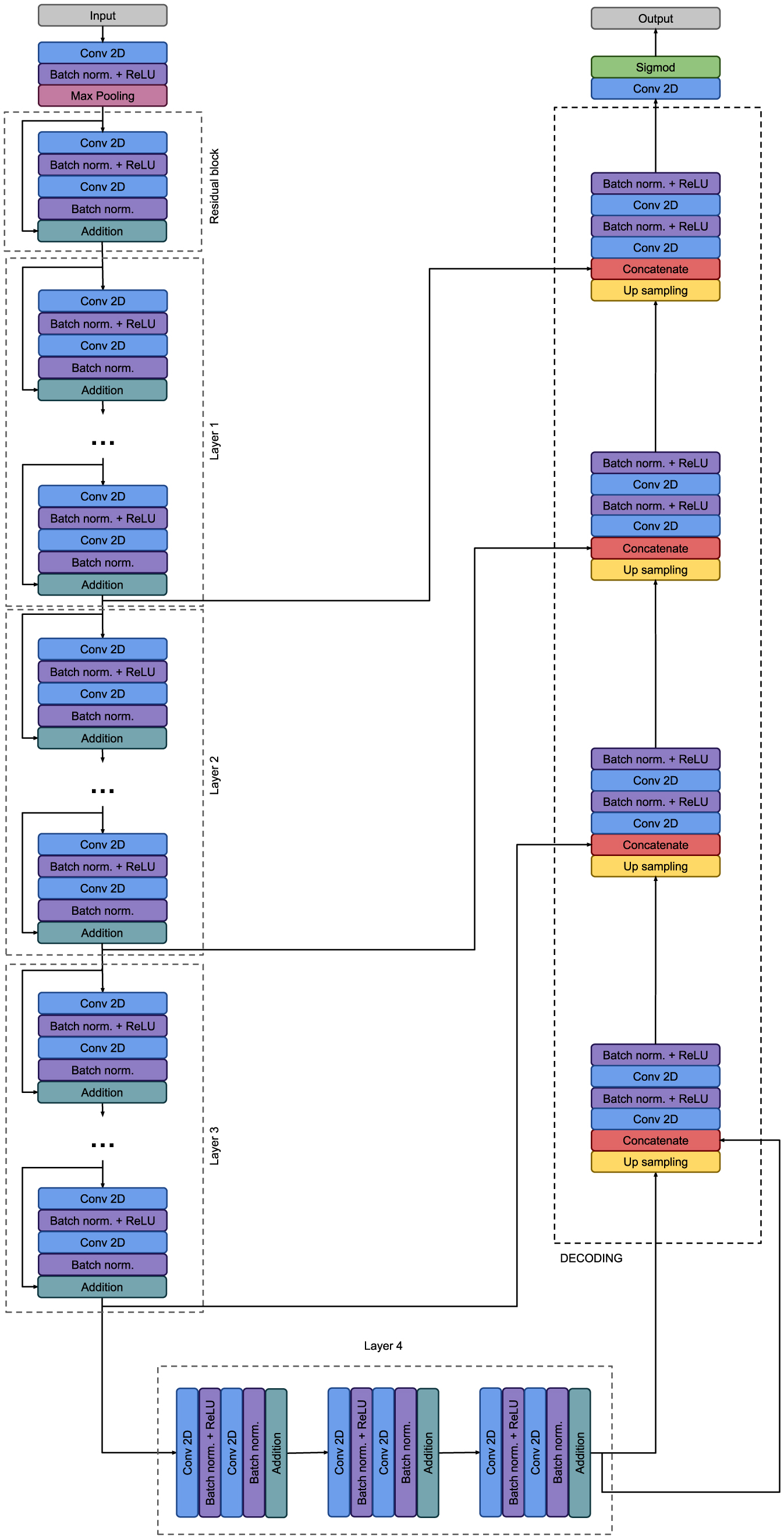
Ultrasound imaging plays a vital role in evaluating thyroid nodules, aiding in the assessment of malignancy risk, monitoring size progression, and serving as a guiding tool for thyroid nodule biopsies. Computer-aided diagnosis (CAD) systems have emerged to assist in diagnosing thyroid lesions, reducing unnecessary biopsies, and contributing to the overall improvement of diagnostic accuracy. The segmentation process plays a crucial role in CAD systems because it marks the region of interest. If segmentation were sufficiently accurate, then it would improve the entire diagnostic process and bring CAD systems closer to routine clinical practice. As far as we know, there are currently only three publicly available datasets of ultrasound images of the thyroid gland that can be used for the purpose of thyroid nodules segmentation. The Thyroid Digital Image Database (TDID) is a long-standing benchmark dataset but faces limitations due to the data ambiguities. The TN3K dataset is more robust than TDID, and the Thyroid Ultrasound Cine-clip dataset offers recent alternatives. In this paper, we implemented a deep learning segmentation model based on UNet with a ResNet encoder. We trained this model on all available data and evaluated it on the TN3K test set. The achieved results for the Dice score, IoU score, accuracy, precision, and recall were 84.24%, 75.48%, 97.24%, 82.75%, and 88.98%, respectively. These results represent the most advanced state-of-the-art scores compared to previously published studies and demonstrate that UNet with a ResNet encoder has the capability to accurately segment thyroid nodules in ultrasound images.

| [1] |
Rahbari R, Zhang L, Kebebew E (2010) Thyroid cancer gender disparity. Future Oncol 6: 1771-1779. https://doi.org/10.2217/fon.10.127 
|
| [2] |
Haugen BR, Alexander EK, Bible KC, et al. (2016) 2015 American Thyroid Association Management Guidelines for adult patients with thyroid nodules and differentiated thyroid cancer: the American Thyroid Association Guidelines task force on thyroid nodules and differentiated thyroid cancer. Thyroid 26: 1-133. https://doi.org/10.1089/thy.2015.0020
|
| [3] |
Tunbridge WM, Evered DC, Hall R, et al. (1977) The spectrum of thyroid disease in a community: the Whickham survey. Clin Endocrinol (Oxf) 7: 481-493. https://doi.org/10.1111/j.1365-2265.1977.tb01340.x
|
| [4] |
Tan GH, Gharib H (1997) Thyroid incidentalomas: management approaches to nonpalpable nodules discovered incidentally on thyroid imaging. Ann Intern Med 126: 226-231. https://doi.org/10.7326/0003-4819-126-3-199702010-00009
|
| [5] |
Guth S, Theune U, Aberle J, et al. (2009) Very high prevalence of thyroid nodules detected by high frequency (13 MHz) ultrasound examination. Eur J Clin Invest 39: 699-706. https://doi.org/10.1111/j.1365-2362.2009.02162.x
|
| [6] |
Remonti LR, Kramer CK, Leitao CB, et al. (2015) Thyroid ultrasound features and risk of carcinoma: a systematic review and meta-analysis of observational studies. Thyroid 25: 538-550. https://doi.org/10.1089/thy.2014.0353
|
| [7] |
Brito JP, Gionfriddo MR, Al Nofal A, et al. (2014) The accuracy of thyroid nodule ultrasound to predict thyroid cancer: systematic review and meta-analysis. J Clin Endocrinol Metab 99: 1253-1263. https://doi.org/10.1210/jc.2013-2928
|
| [8] |
Tessler FN, Middleton WD, Grant EG, et al. (2017) ACR Thyroid Imaging, Reporting and Data System (TI-RADS): white paper of the ACR TI-RADS committee. J Am Coll Radiol 14: 587-595. https://doi.org/10.1016/j.jacr.2017.01.046
|
| [9] |
Zhu YC, AlZoubi A, Jassim S, et al. (2021) A generic deep learning framework to classify thyroid and breast lesions in ultrasound images. Ultrasonics 110: 106300. https://doi.org/10.1016/j.ultras.2020.106300
|
| [10] |
Chi J, Walia E, Babyn P, et al. (2017) Thyroid nodule classification in ultrasound images by fine-tuning deep convolutional neural network. J Digit Imaging 30: 477-486. https://doi.org/10.1007/s10278-017-9997-y
|
| [11] |
Mei X, Dong X, Deyer T, et al. (2017) Thyroid nodule benignty prediction by deep feature extraction. 2017 IEEE 17th International Conference on Bioinformatics and Bioengineering (BIBE) . Washington, DC, USA: 241-245. https://doi.org/10.1109/BIBE.2017.00-48
|
| [12] |
Liu T, Xie S, Yu J, et al. (2017) Classification of thyroid nodules in ultrasound images using deep model based transfer learning and hybrid features. 2017 IEEE International Conference on Acoustics, Speech and Signal Processing (ICASSP) . New Orleans, LA, USA: 919-923. https://doi.org/109/ICASSP.2017.7952290
|
| [13] |
Prochazka A, Gulati S, Holinka S, et al. (2019) Patch-based classification of thyroid nodules in ultrasound images using direction independent features extracted by two-threshold binary decomposition. Comput Med Imaging Graph 71: 9-18. https://doi.org/10.1016/j.compmedimag.2018.10.001
|
| [14] |
Prochazka A, Gulati S, Holinka S, et al. (2019) Classification of thyroid nodules in ultrasound images using direction-independent features extracted by two-threshold binary decomposition. Technol Cancer Res Treat 18. https://doi.org/10.1177/1533033819830748
|
| [15] |
Chen J, You H, Li K (2020) A review of thyroid gland segmentation and thyroid nodule segmentation methods for medical ultrasound images. Comput Methods Programs Biomed 185: 105329. https://doi.org/10.1016/j.cmpb.2020.105329
|
| [16] |
Gong H, Chen J, Chen G, et al. (2023) Thyroid region prior guided attention for ultrasound segmentation of thyroid nodules. Comput Biol Med 155: 106389. https://doi.org/10.1016/j.compbiomed.2022.106389
|
| [17] |
Pan H, Zhou Q, Latecki LJ (2021) SGUNET: Semantic guided UNET for thyroid nodule segmentation. 2021 IEEE 18th International Symposium on Biomedical Imaging (ISBI) . Nice, France: 630-634. https://doi.org/10.1109/ISBI48211.2021.9434051
|
| [18] |
Li C, Du R, Luo Q, et al. (2023) A novel model of thyroid nodule segmentation for ultrasound images. Ultrasound Med Biol 49: 489-496. https://doi.org/10.1016/j.ultrasmedbio.2022.09.017
|
| [19] |
Wang R, Zhou H, Fu P, et al. (2023) A multiscale attentional unet model for automatic segmentation in medical ultrasound images. Ultrason Imaging 45: 159-174. https://doi.org/10.1177/01617346231169789
|
| [20] | Pedraza L, Vargas C, Narvaez F, et al. (2015) An open access thyroid ultrasound-image Database. 10th International Symposium on Medical Information Processing and Analysis . https://doi.org/10.1117/12.2073532 |
| [21] |
Ma J, Wu F, Jiang T, et al. (2017) Ultrasound image-based thyroid nodule automatic segmentation using convolutional neural networks. Int J Comput Assist Radiol Surg 12: 1895-1910. https://doi.org/10.1007/s11548-017-1649-7
|
| [22] | Ying X, Yu Z, Yu R, et al. (2018) Thyroid nodule segmentation in ultrasound images based on cascaded convolutional neural network. Neural Information Processing . Cham: Springer 373-384. https://doi.org/10.1007/978-3-030-04224-0_32 |
| [23] | Ronneberger O, Fischer P, Brox T (2015) U-Net: Convolutional networks for biomedical image segmentation. Medical Image Computing and Computer-Assisted Intervention – MICCAI 2015 . Cham: Springer 234-241. https://doi.org/10.1007/978-3-319-24574-4_28 |
| [24] | Simonyan K, Zisserman A (2014). https://doi.org/10.48550/arXiv.1409.1556 |
| [25] |
Kumar V, Webb J, Gregory A, et al. (2020) Automated segmentation of thyroid nodule, gland, and cystic components from ultrasound images using deep learning. IEEE Access 8: 63482-63496. https://doi.org/10.1109/ACCESS.2020.2982390
|
| [26] |
Sun J, Li C, Lu Z, et al. (2022) TNSNet: Thyroid nodule segmentation in ultrasound imaging using soft shape supervision. Comput Meth Prog Bio 215: 106600. https://doi.org/10.1016/j.cmpb.2021.106600
|
| [27] |
Song R, Zhu C, Zhang L, et al. (2022) Dual-branch network via pseudo-label training for thyroid nodule detection in ultrasound image. Appl Intell 52: 11738-11754. https://doi.org/10.1007/s10489-021-02967-2
|
| [28] |
Gomes Ataide E, Agrawal S, Jauhari A, et al. (2021) Comparison of deep learning algorithms for semantic segmentation of ultrasound thyroid nodules. Curr Dir Biomed Eng 7: 879-882. https://doi.org/10.1515/cdbme-2021-2224
|
| [29] |
Niu K, Guo Z, Peng X, et al. (2022) P-ResUnet: Segmentation of brain tissue with Purified Residual Unet. Comput Biol Med 151: 106294. https://doi.org/10.1016/j.compbiomed.2022.106294
|
| [30] |
Diakogiannis FI, Waldner F, Caccetta P, et al. (2020) ResUNet-a: A deep learning framework for semantic segmentation of remotely sensed data. Isprs J Photogramm Remote Sens 162: 94-114. https://doi.org/10.1016/j.isprsjprs.2020.01.013
|
| [31] | Wang JJ, Gao J, Ren JW, et al. (2021) DFP-ResUNet: Convolutional neural network with a dilated convolutional feature pyramid for multimodal brain tumor segmentation. Comput Meth Prog Biomed 208. https://doi.org/10.1016/j.cmpb.2021.106208 |
| [32] |
Morelli R, Clissa L, Amici R, et al. (2021) Automating cell counting in fluorescent microscopy through deep learning with c-ResUnet. Sci Rep 11. https://doi.org/10.1038/s41598-021-01929-5
|
| [33] |
Sabir MW, Khan Z, Saad NM, et al. (2022) Segmentation of liver tumor in CT scan using ResU-Net. Appl Sci 12. https://doi.org/10.3390/app12178650
|
| [34] | Wang R, Shen H, Zhou M (2019) Ultrasound nerve segmentation of brachial plexus based on optimized ResU-Net. 2019 IEEE International Conference on Imaging Systems & Techniques (IST) . https://doi.org/10.1109/IST48021.2019.9010317 |
| [35] |
Cai L, Li Q, Zhang J, et al. (2023) Ultrasound image segmentation based on Transformer and U-Net with joint loss. PeerJ Comput Sci 9: e1638. https://doi.org/10.7717/peerj-cs.1638
|
| [36] |
Song SH, Han JH, Kim KS, et al. (2022) Deep-learning segmentation of ultrasound images for automated calculation of the hydronephrosis area to renal parenchyma ratio. Investig Clin Urol 63: 455-463. https://doi.org/10.4111/icu.20220085
|
| [37] | Chen J, Lu Y, Yu Q, et al. Transunet: Transformers make strong encoders for medical image segmentation (2021). https://doi.org/10.48550/arXiv.2102.04306 |
| [38] |
Chouiha B, Amamra A (2021) Thyroid Nodules Recognition in ultrasound images based on ImageNet top-performing deep convolutional neural networks. Advances in Computing Systems and Applications . Cham: Springer 313-322. https://doi.org/10.1007/978-3-030-69418-0_28
|
| [39] |
Gomes Ataide EJ, Ponugoti N, Illanes A, et al. (2020) Thyroid nodule classification for physician decision support using machine learning-evaluated geometric and morphological features. Sensors 20. https://doi.org/10.3390/s20216110
|
| [40] |
Buslaev A, Iglovikov VI, Khvedchenya E, et al. (2020) Albumentations: Fast and flexible image augmentations. Information 11. https://doi.org/10.3390/info11020125
|
| [41] | Loshchilov I, Hutter F Sgdr: Stochastic gradient descent with warm restarts (2016). https://doi.org/10.48550/arXiv.1608.03983 |
| [42] |
Gong H, Chen G, Wang R, et al. (2021) Multi-task learning for thyroid nodule segmentation with thyroid region prior. 2021 IEEE 18th International Symposium on Biomedical Imaging (ISBI) . Nice, France: 257-261. https://doi.org/10.1109/ISBI48211.2021.9434087
|
| [43] | Long J, Shelhamer E, Darrell T (2015) Fully convolutional networks for semantic segmentation. IEEE Trans Pattern Anal Mach Intell 39: 640-651. https://doi.org/10.1109/TPAMI.2016.2572683 |
| [44] |
Badrinarayanan V, Kendall A, Cipolla R (2017) Segnet: A deep convolutional encoder-decoder architecture for image segmentation. IEEE Trans Pattern Anal Mach Intell 39: 2481-2495. https://doi.org/10.1109/TPAMI.2016.2644615
|
| [45] | Chen LC, Zhu Y, Papandreou G, et al. (2018) Encoder-decoder with atrous separable convolution for semantic image segmentation. Computer Vision – ECCV 2018 . Cham: Springer 833-851. https://doi.org/10.1007/978-3-030-01234-2_49 |
| [46] | Feng S, Zhao H, Shi F, et al. (2020) CPFNet: Context pyramid fusion network for medical image segmentation. IEEE Trans Med Imaging 39: 3008-3018. https://doi.org/10.1109/TMI.2020.2983721 |
| [47] | Brauer VFH, Eder P, Miehle K, et al. (2005) Interobserver variation for ultrasound determination of thyroid nodule volumes. Thyroid 15: 1169-1175. https://doi.org/10.1089/thy.2005.15.1169 |
| [48] |
Lee HJ, Yoon DY, Seo YL, et al. (2018) Intraobserver and interobserver variability in ultrasound measurements of thyroid nodules. J Ultrasound Med 37: 173-178. https://doi.org/10.1002/jum.14316
|
| [49] |
Özgen A, Erol C, Kaya A, et al. (1999) Interobserver and intraobserver variations in sonographic measurement of thyroid volume in children. Eur J Endocrinol 140: 328-331. https://doi.org/10.1530/eje.0.1400328
|
 medsci-12-02-009-s001.pdf medsci-12-02-009-s001.pdf |
 |


Figures(5) / Tables(4)

Antonin Prochazka, Jan Zeman. Thyroid nodule segmentation in ultrasound images using U-Net with ResNet encoder: achieving state-of-the-art performance on all public datasets[J]. AIMS Medical Science, 2025, 12(2): 124-144. doi: 10.3934/medsci.2025009


 DownLoad: