The study aimed to evaluate the impact of the early addition of a Saccharomyces cerevisiae HD A54 strain before pressing during winemaking. This approach aimed to reduce the dissolved oxygen in the grape must, thus preserving the wine characteristics. Two different treatments were settled: Trial A, where sulphite or other substances were not added during pressing; and Trial B, where a S. cerevisiae strain was added at the pressing stage. The chemical parameters were determined through an enzymatic analyzer, which indicated a faster fructose consumption compared to the glucose in Trial A. The plate counts were measured to monitor the microbial groups during vinification. Both treatments showed regular trends with respect to the Saccharomyces population. Trial B exhibited a higher oxygen consumption compared to the control trial, especially in the early stages of winemaking. This was determined through a dissolved O2 analysis. Furthermore, Trial B had lower absorbance values at the post-pressing and pre-clarification stages. Both the dissolved oxygen and the absorbance analyses underscored the positive impact of the S. cerevisiae HD A54 strain in protecting against oxidative processes in the grape musts at the pre-fermentative stage. The analysis of volatile organic compounds detected 30 different compounds, including alcohols and esters. Trial B had higher alcohol levels, particularly hydroxyethylbenzene (135.31 mg/L vs. 44.23 mg/L in Trial A). Trial A had almost a four times higher ethyl acetate concentration than Trial B, which is an indicator of oxidation. Interestingly, Trial B showed higher concentrations of 3-methyl-butyl acetate and 2-phenylethyl acetate, which are molecules that correspond to fruity (banana) and floreal (rose) aromas, respectively. Regarding the sensory analysis, Trial B received better scores for the fruity and floral attributes, as well as the overall wine quality.
Citation: Enrico Viola, Vincenzo Naselli, Rosario Prestianni, Antonino Pirrone, Antonella Porrello, Filippo Amato, Riccardo Savastano, Antonella Maggio, Micaela Carusi, Venera Seminerio, Valentina Craparo, Azzurra Vella, Davide Alongi, Luca Settanni, Giuseppe Notarbartolo, Nicola Francesca, Antonio Alfonzo. The impact of a Saccharomyces cerevisiae bio-protective strain during cold static clarification on Catarratto wine[J]. AIMS Microbiology, 2025, 11(1): 40-58. doi: 10.3934/microbiol.2025003
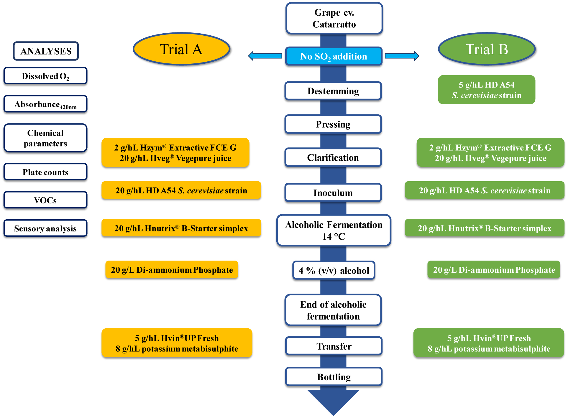
The study aimed to evaluate the impact of the early addition of a Saccharomyces cerevisiae HD A54 strain before pressing during winemaking. This approach aimed to reduce the dissolved oxygen in the grape must, thus preserving the wine characteristics. Two different treatments were settled: Trial A, where sulphite or other substances were not added during pressing; and Trial B, where a S. cerevisiae strain was added at the pressing stage. The chemical parameters were determined through an enzymatic analyzer, which indicated a faster fructose consumption compared to the glucose in Trial A. The plate counts were measured to monitor the microbial groups during vinification. Both treatments showed regular trends with respect to the Saccharomyces population. Trial B exhibited a higher oxygen consumption compared to the control trial, especially in the early stages of winemaking. This was determined through a dissolved O2 analysis. Furthermore, Trial B had lower absorbance values at the post-pressing and pre-clarification stages. Both the dissolved oxygen and the absorbance analyses underscored the positive impact of the S. cerevisiae HD A54 strain in protecting against oxidative processes in the grape musts at the pre-fermentative stage. The analysis of volatile organic compounds detected 30 different compounds, including alcohols and esters. Trial B had higher alcohol levels, particularly hydroxyethylbenzene (135.31 mg/L vs. 44.23 mg/L in Trial A). Trial A had almost a four times higher ethyl acetate concentration than Trial B, which is an indicator of oxidation. Interestingly, Trial B showed higher concentrations of 3-methyl-butyl acetate and 2-phenylethyl acetate, which are molecules that correspond to fruity (banana) and floreal (rose) aromas, respectively. Regarding the sensory analysis, Trial B received better scores for the fruity and floral attributes, as well as the overall wine quality.

| [1] |
Ferrer-Gallego R, Puxeu M, Nart E, et al. (2017) Evaluation of Tempranillo and Albariño SO2-free wines produced by different chemical alternatives and winemaking procedures. Food Res Int 102: 647-657. https://doi.org/10.1016/j.foodres.2017.09.046 
|
| [2] |
Guerrero RF, Cantos-Villar E (2015) Demonstrating the efficiency of sulphur dioxide replacements in wine: A parameter review. Trends Food Sci Technol 42: 27-43. https://doi.org/10.1016/j.tifs.2014.11.004
|
| [3] |
Christofi S, Malliaris D, Katsaros G, et al. (2020) Limit SO2 content of wines by applying High Hydrostatic Pressure. Innov Food Sci Emerg Technol 62: 102342. https://doi.org/10.1016/j.ifset.2020.102342
|
| [4] |
Santos MC, Nunes C, Cappelle J, et al. (2013) Effect of high pressure treatments on the physicochemical properties of a sulphur dioxide-free red wine. Food Chem 141: 2558-2566. https://doi.org/10.1016/j.foodchem.2013.05.022
|
| [5] |
Roullier-Gall C, Hemmler D, Gonsior M, et al. (2017) Sulfites and the wine metabolome. Food Chem 237: 106-113. https://doi.org/10.1016/j.foodchem.2017.05.039
|
| [6] |
Di Gianvito P, Englezos V, Rantsiou K, et al. (2022) Bioprotection strategies in winemaking. Int J Food Microbiol 364: 109532. https://doi.org/10.1016/j.ijfoodmicro.2022.109532
|
| [7] |
Ferraz P, Cassio F, Lucas C (2019) Potential of yeasts as biocontrol agents of the phytopathogen causing cacao witches' broom disease: Is microbial warfare a solution?. Front Microbiol 10: 1766. https://doi.org/10.3389/fmicb.2019.01766
|
| [8] |
Keswani C, Singh HB, Hermosa R, et al. (2019) Antimicrobial secondary metabolites from agriculturally important fungi as next biocontrol agents. Appl Microbiol Biotechnol 103: 9287-9303. https://doi.org/10.1007/s00253-019-10209-2103
|
| [9] | OIV (International Organisation of Vine and Wine)Recueil des methodes internationales d'analyses des vins et des moûts (2010). Avaible from: https://www.oiv.int/fr/normes-et-documents-techniques/methodes-danalyse/recueil-des-methodes-internationales-danalyse-des-vins-et-des-mouts-2-vol |
| [10] | Directive 2003/89/EC of the European parliament and of the council amending directive 2000/13/EC as regards indication of the ingredients present in foodstuffs. Avaible from: http://data.europa.eu/eli/dir/2003/89/oj |
| [11] |
Lisanti MT, Blaiotta G, Nioi C, et al. (2019) Alternative methods to SO2 for microbiological stabilization of wine. Compr Rev Food Sci Food Saf 18: 455-479. https://doi.org/10.1111/1541-4337.12422
|
| [12] |
Silva M, Gama J, Pinto N, et al. (2019) Sulfite concentration and the occurrence of headache in young adults: A prospective study. Eur J Clin Nutr 73: 1316-1322. https://doi.org/10.1038/s41430-019-0420-2
|
| [13] |
Santos MC, Nunes C, Rocha MAM, et al. (2015) High pressure treatments accelerate changes in volatile composition of sulphur dioxide-free wine during bottle storage. Food Chem 188: 406-414. https://doi.org/10.1016/j.foodchem.2015.05.002
|
| [14] |
Fredericks IN, du Toit M, Krügel M (2011) Efficacy of ultraviolet radiation as an alternative technology to inactivate microorganisms in grape juices and wines. Food Microbiol 28: 510-517. https://doi.org/10.1016/j.fm.2010.10.018
|
| [15] |
Pandin C, Le Coq D, Canette A, et al. (2017) Should the biofilm mode of life be taken into consideration for microbial biocontrol agents?. Microb Biotechnol 10: 719-734. https://doi.org/10.1111/1751-7915.12693
|
| [16] |
Bauer MA, Kainz K, Carmona-Gutierrez D, et al. (2018) Microbial wars: Competition in ecological niches and within the microbiome. Microb Cell 5: 215. https://doi.org/10.15698/mic2018.05.628
|
| [17] |
Parijs I, Steenackers HP (2018) Competitive inter-species interactions underlie the increased antimicrobial tolerance in multispecies brewery biofilms. ISME J 12: 2061-2075. https://doi.org/10.1038/s41396-018-0146-5
|
| [18] |
Ghoul M, Mitri S (2016) The ecology and evolution of microbial competition. Trends Microbiol 24: 833-845. https://doi.org/10.1016/j.tim.2016.06.011
|
| [19] |
Curiel JA, Morales P, Gonzalez R, et al. (2017) Different non-Saccharomyces yeast species stimulate nutrient consumption in Saccharomyces cerevisiae mixed cultures. Front Microbiol 8: 2121. https://doi.org/10.3389/fmicb.2017.02121
|
| [20] |
Petitgonnet C, Klein GL, Roullier-Gall C, et al. (2019) Influence of cell-cell contact between L. thermotolerans and S. cerevisiae on yeast interactions and the exo-metabolome. Food Microbiol 83: 122-133. https://doi.org/10.1016/j.fm.2019.05.005
|
| [21] |
Prior KJ, Bauer FF, Divol B (2019) The utilisation of nitrogenous compound by commercial non-Saccharomyces yeasts associated with wine. Food Microbiol 79: 75-84. https://doi.org/10.1016/j.fm.2018.12.002
|
| [22] |
Siedler S, Balti R, Neves AR (2019) Bioprotective mechanisms of lactic acid bacteria against fungal spoilage of food. Curr Opin Biotechnol 56: 138-146. https://doi.org/10.1016/j.copbio.2018.11.015
|
| [23] |
Pallmann CL, Brown JA, Olineka TL, et al. (2001) Use of WL medium to profile native flora fermentations. Am J Enol Vitic 52: 198-203. http://dx.doi.org/10.5344/ajev.2001.52.3.198
|
| [24] |
Couto MB, Reizinho RG, Duarte FL (2005) Partial 26S rDNA restriction analysis as a tool to characterise non-Saccharomyces yeasts present during red wine fermentations. Int J Food Microbiol 102: 49-56. https://doi.org/10.1016/j.ijfoodmicro.2005.01.005
|
| [25] | ISO 15214Microbiology of food and animal feeding stuffs–Horizontal method for the enumeration of mesophilic lactic acid bacteria–Colony-count technique at 30 °C (1998). |
| [26] | OIV (International Organisation of Vine and Wine)Compendium of international methods of wine and must analysis (2020). Available from: https://www.oiv.int/en/technical-standards-and-documents/methods-of-analysis/compendium-of-international-methods-of-analysis-of-wines-and-musts-2-vol |
| [27] | OIV (International Organisation of Vine and Wine)Compendium of international methods of wine and must analysis (2020). Available from: https://www.oiv.int/en/technical-standards-and-documents/methods-of-analysis/compendium-of-international-methods-of-analysis-of-wines-and-musts-2-vol |
| [28] |
Matraxia M, Alfonzo A, Prestianni R, et al. (2021) Non-conventional yeasts from fermented honey by-products: Focus on Hanseniaspora uvarum strains for craft beer production. Food Microbiol 99: 103806. https://doi.org/10.1016/j.fm.2021.103806
|
| [29] |
Chawafambira A (2021) The effect of incorporating herbal (Lippia javanica) infusion on the phenolic, physicochemical, and sensorial properties of fruit wine. Food Sci Nutr 9: 4539-4549. https://doi.org/10.1002/fsn3.2432
|
| [30] |
Francesca N, Naselli V, Prestianni R, et al. (2024) Impact of two new non-conventional yeasts, Candida oleophila and Starmerella lactis-condensi, isolated from sugar-rich substrates, on Frappato wine aroma. Food Biosci 57: 103500. https://doi.org/10.1016/j.fbio.2023.103500
|
| [31] | Jackson RS (2016) Wine Tasting: A Professional Handbook. Boston: Academic Press. |
| [32] |
Issa-Issa H, Guclu G, Noguera-Artiaga L, et al. (2020) Aroma-active compounds, sensory profile, and phenolic composition of Fondillón. Food Chem 316: 126353. https://doi.org/10.1016/j.foodchem.2020.126353
|
| [33] |
Cochran WG, Cox GM (1957) Experimental designs. New York: John Wiley & Sons. |
| [34] |
Di Maro E, Ercolini D, Coppola S (2007) Yeast dynamics during spontaneous wine fermentation of the Catalanesca grape. Int J Food Microbiol 117: 201-210. https://doi.org/10.1016/j.ijfoodmicro.2007.04.007
|
| [35] |
Varela C, Sengler F, Solomon M, et al. (2016) Volatile flavour profile of reduced alcohol wines fermented with the non-conventional yeast species Metschnikowia pulcherrima and Saccharomyces uvarum. Food Chem 209: 57-64. https://doi.org/10.1016/j.foodchem.2016.04.024
|
| [36] | González SS, Barrio E, Querol A (2007) Molecular identification and characterization of wine yeasts isolated from Tenerife (Canary Island, Spain). J Appl Microbiol 102: 1018-1025. https://doi.org/10.1111/j.1365-2672.2006.03150.x |
| [37] |
Sannino C, Francesca N, Corona O, et al. (2013) Effect of the natural winemaking process applied at industrial level on the microbiological and chemical characteristics of wine. J Biosci Bioeng 116: 347-356. https://doi.org/10.1016/j.jbiosc.2013.03.005
|
| [38] |
Minebois R, Pérez-Torrado R, Querol A (2020) A time course metabolism comparison among Saccharomyces cerevisiae, S. uvarum and S. kudriavzevii species in wine fermentation. Food Microbiol 90: 103484. https://doi.org/10.1016/j.fm.2020.103484
|
| [39] |
Morgan SC, Haggerty JJ, Johnston B, et al. (2019) Response to sulfur dioxide addition by two commercial Saccharomyces cerevisiae strains. Fermentation 5: 69. https://doi.org/10.3390/fermentation5030069
|
| [40] |
Csoma H, Kállai Z, Czentye K, et al. (2023) Starmerella lactis-condensi, a yeast that has adapted to the conditions in the oenological environment. Int J Food Microbiol 401: 110282. https://doi.org/10.1016/j.ijfoodmicro.2023.110282
|
| [41] |
Alfonzo A, Prestianni R, Gaglio R, et al. (2021) Effects of different yeast strains, nutrients and glutathione-rich inactivated yeast addition on the aroma characteristics of Catarratto wines. Int J Food Microbiol 360: 109325. https://doi.org/10.1016/j.ijfoodmicro.2021.109325
|
| [42] |
Windholtz S, Nioi C, Coulon J, et al. (2023) Bioprotection by non-Saccharomyces yeasts in oenology: Evaluation of O2 consumption and impact on acetic acid bacteria. Int J Food Microbiol 405: 110338. https://doi.org/10.1016/j.ijfoodmicro.2023.110338
|
| [43] | Catarino A, Alves S, Mira H (2014) Influence of technological operations in the dissolved oxygen content of wines. J Chem Chem Eng 8: 390-394. https://doi.org/10.17265/1934-7375%2F2014.04.010 |
| [44] |
Darias-Martı́n J, Dı́az-González D, Dı́az-Romero C (2004) Influence of two pressing processes on the quality of must in white wine production. J Food Eng 63: 335-340. https://doi.org/10.1016/j.jfoodeng.2003.08.005
|
| [45] |
Villano D, Fernández-Pachón MS, Troncoso AM, et al. (2006) Influence of enological practices on the antioxidant activity of wines. Food Chem 95: 394-404. https://doi.org/10.1016/j.foodchem.2005.01.005
|
| [46] |
Selli S, Cabaroglu T, Canbas A, et al. (2004) Volatile composition of red wine from cv. Kalecik Karasι grown in central Anatolia. Food Chem 85: 207-213. https://doi.org/10.1016/j.foodchem.2003.06.008
|
| [47] |
Cañas PI, Romero EG, Alonso SG, et al. (2008) Changes in the aromatic composition of Tempranillo wines during spontaneous malolactic fermentation. J Food Compos Anal 21: 724-730. https://doi.org/10.1016/j.jfca.2007.12.005
|
| [48] |
Fariña L, Villar V, Ares G, et al. (2015) Volatile composition and aroma profile of Uruguayan Tannat wines. Food Res Int 69: 244-255. https://doi.org/10.1016/j.foodres.2014.12.029
|
| [49] |
De Lerma NL, Bellincontro A, Mencarelli F, et al. (2012) Use of electronic nose, validated by GC–MS, to establish the optimum off-vine dehydration time of wine grapes. Food Chem 130: 447-452. https://doi.org/10.1016/j.foodchem.2011.07.058
|
| [50] | Li H (2006) Wine Tasting. Beijing: China Science Press 29-106. |
| [51] |
Li H, Tao YS, Wang H, et al. (2008) Impact odorants of Chardonnay dry white wine from Changli County (China). Eur Food Res Technol 227: 287-292. https://doi.org/10.1007/s00217-007-0722-9
|
| [52] |
Ferreira V, López R, Cacho JF (2000) Quantitative determination of the odorants of young red wines from different grape varieties. J Sci Food Agric 80: 1659-1667. https://doi.org/10.1002/1097-0010(20000901)80:11%3C1659::AID-JSFA693%3E3.0.CO;2-6
|
| [53] |
Gómez-Míguez MJ, Cacho JF, Ferreira V, et al. (2007) Volatile components of Zalema white wines. Food Chem 100: 1464-1473. https://doi.org/10.1016/j.foodchem.2005.11.045
|
| [54] |
Guth H (1997) Quantitation and sensory studies of character impact odorants of different white wine varieties. J Agric Food Chem 45: 3027-3032. https://doi.org/10.1021/jf970280a
|
| [55] |
Rocha SM, Rodrigues F, Coutinho P, et al. (2004) Volatile composition of Baga red wine: Assessment of the identification of the would-be impact odourants. Anal Chim Acta 513: 257-262. https://doi.org/10.1016/j.aca.2003.10.009
|
| [56] | Lloret A, Boido E, Lorenzo D, et al. (2002) Aroma variation in Tannat wines: Effect of malolactic fermentation on ethyl lactate level and its enantiomeric distribution. Ital J Food Sci 14: 175-180. http://hdl.handle.net/10449/18119 |
| [57] |
Delgado JA, Sánchez-Palomo E, Alises MO, et al. (2022) Chemical and sensory aroma typicity of La Mancha Petit Verdot wines. LWT 162: 113418. https://doi.org/10.1016/j.lwt.2022.113418
|
| [58] |
Yao M, Wang F, Arpentin G (2023) Bioprotection as a tool to produce natural wine: Impact on physicochemical and sensory analysis. BIO Web Conf 56: 02019. https://doi.org/10.1051/bioconf/20235602019
|
| [59] |
Bayram M, Kayalar M (2018) White wines from Narince grapes: Impact of two different grape provenances on phenolic and volatile composition. OENO One 52: 81-92. https://doi.org/10.20870/oeno-one.2018.52.2.2114
|
| [60] |
Zoecklein BW, Fugelsang KC, Gump BH, et al. (1995) Volatile acidity. Wine Analysis and Production . New York: Springer 192-198. https://doi.org/10.1007/978-1-4757-6978-4_11
|
| [61] |
Canonico L, Comitini F, Ciani M (2019) Metschnikowia pulcherrima selected strain for ethanol reduction in wine: Influence of cell immobilization and aeration condition. Foods 8: 378. https://doi.org/10.3390%2Ffoods8090378
|
| [62] |
Laguna L, Sarkar A, Bryant MG, et al. (2017) Exploring mouthfeel in model wines: Sensory-to-instrumental approaches. Food Res Int 102: 478-486. https://doi.org/10.1016/j.foodres.2017.09.009
|


Figures(6) / Tables(2)

Enrico Viola, Vincenzo Naselli, Rosario Prestianni, Antonino Pirrone, Antonella Porrello, Filippo Amato, Riccardo Savastano, Antonella Maggio, Micaela Carusi, Venera Seminerio, Valentina Craparo, Azzurra Vella, Davide Alongi, Luca Settanni, Giuseppe Notarbartolo, Nicola Francesca, Antonio Alfonzo. The impact of a Saccharomyces cerevisiae bio-protective strain during cold static clarification on Catarratto wine[J]. AIMS Microbiology, 2025, 11(1): 40-58. doi: 10.3934/microbiol.2025003


 DownLoad: