Exposure to laboratory animal allergens has been a significant cause of IgE-mediated allergic symptoms and occupational asthma (OA). Mice are the predominant species used in medical and scientific facilities. We have previously published a review of our air monitoring data of mouse and rat major allergens (mus m 1 and rat n 1) expressible in ng·m−3 from 2005–2016. We have now reassessed all this largely United Kingdom (UK) air monitoring data from 2005–2022, which include 77% and 47% additional mouse and rat results, respectively. Where possible, we have categorized the results to specific tasks and areas to identify those associated with higher exposures and explored temporal trends in exposure together with an estimation of the annual incidence of OA in 2005 and 2018. A downward shift in mouse results for personal samples was apparent from 2014, with evidence of a decrease in the 90th percentile, but both personal and static rat samples confoundingly showed an apparent increase from 2017. Activities of “cage changing”, “cage cleaning”, and “cage washing, dirty side” suggested substantial personal exposures in some facilities, while “bedding dumping” and “cage scraping” suggested generally high exposures, albeit modified by any respiratory protective equipment worn. Individually ventilated cages reduce exposure, but filter changing/cleaning can still lead to high exposures. Exposure from experimental and husbandry duties were generally lower, but in some facilities activities where animals are handled outside of cages can cause significant exposures. The reduction in personal exposure to the predominant species is consistent with an estimated 55% decrease in the UK annual incidence rate of OA in 2018 from 2005. The data may help facilities to improve exposure control by identifying higher risk activities, benchmarking their own monitoring data and help further reduce the risk of sensitization and subsequent allergic respiratory ill-health.
Citation: Howard Mason, Kate Jones. Airborne exposure to laboratory animal allergens: 2005–2022[J]. AIMS Allergy and Immunology, 2024, 8(1): 18-33. doi: 10.3934/Allergy.2024003
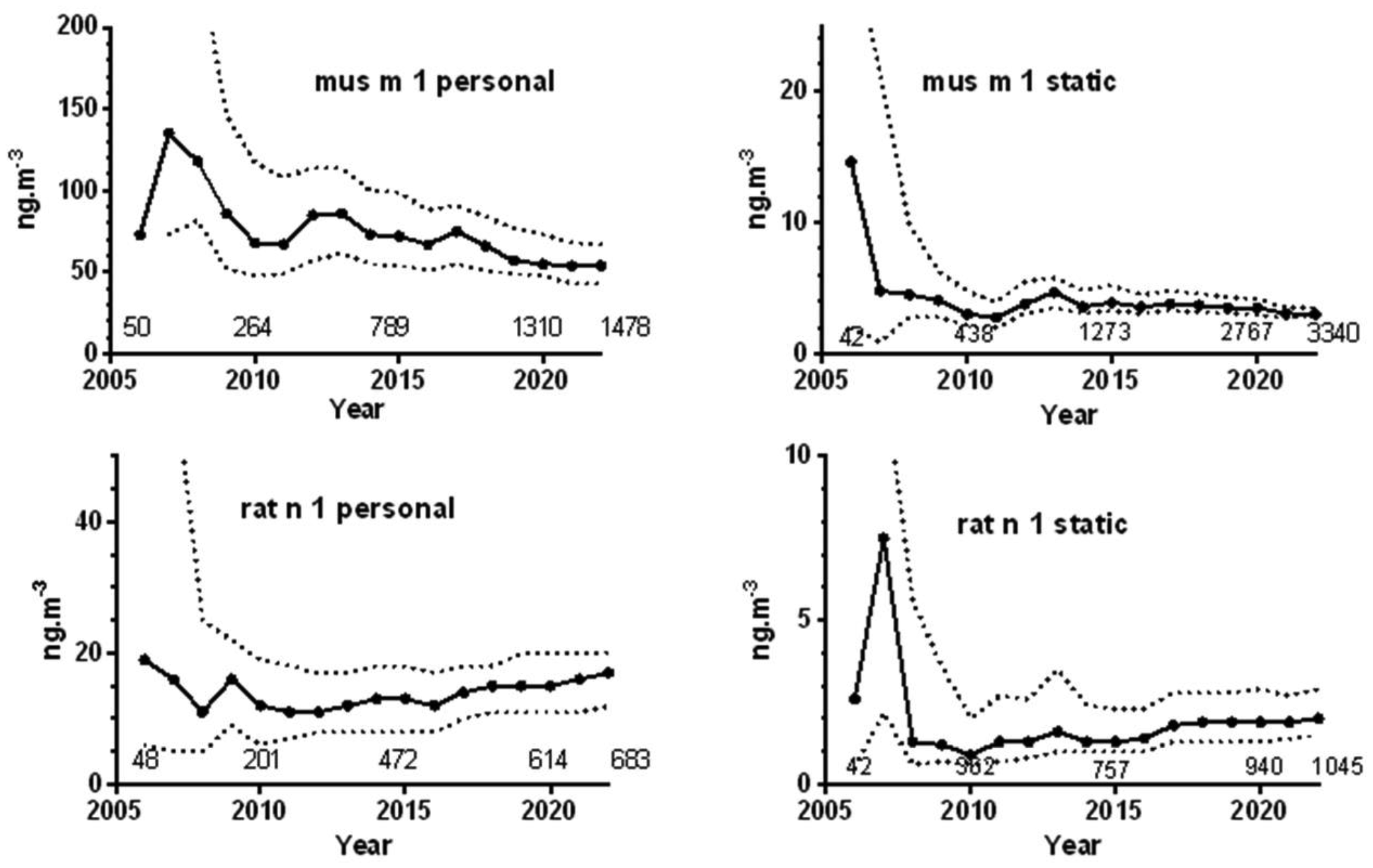
Exposure to laboratory animal allergens has been a significant cause of IgE-mediated allergic symptoms and occupational asthma (OA). Mice are the predominant species used in medical and scientific facilities. We have previously published a review of our air monitoring data of mouse and rat major allergens (mus m 1 and rat n 1) expressible in ng·m−3 from 2005–2016. We have now reassessed all this largely United Kingdom (UK) air monitoring data from 2005–2022, which include 77% and 47% additional mouse and rat results, respectively. Where possible, we have categorized the results to specific tasks and areas to identify those associated with higher exposures and explored temporal trends in exposure together with an estimation of the annual incidence of OA in 2005 and 2018. A downward shift in mouse results for personal samples was apparent from 2014, with evidence of a decrease in the 90th percentile, but both personal and static rat samples confoundingly showed an apparent increase from 2017. Activities of “cage changing”, “cage cleaning”, and “cage washing, dirty side” suggested substantial personal exposures in some facilities, while “bedding dumping” and “cage scraping” suggested generally high exposures, albeit modified by any respiratory protective equipment worn. Individually ventilated cages reduce exposure, but filter changing/cleaning can still lead to high exposures. Exposure from experimental and husbandry duties were generally lower, but in some facilities activities where animals are handled outside of cages can cause significant exposures. The reduction in personal exposure to the predominant species is consistent with an estimated 55% decrease in the UK annual incidence rate of OA in 2018 from 2005. The data may help facilities to improve exposure control by identifying higher risk activities, benchmarking their own monitoring data and help further reduce the risk of sensitization and subsequent allergic respiratory ill-health.
health and safety executive
individually ventilated cages
laboratory animal allergens
limit of detection
occupational asthma
respiratory protective equipment

| [1] | NC3Rs, National Centre for the Replacement Refinement and Reduction of Animals for Research. NC3Rs (2024). Available from: https://nc3rs.org.uk/ |
| [2] | Home Office, Annual Statistics of Scientific Procedures on Living Animals Great Britain 2019. GOV.UK (2019). Available from: https://www.gov.uk/government/statistics/statistics-of-scientific-procedures-on-living-animals-great-britain-2019 |
| [3] | Home Office, Annual Statistics of Scientific Procedures on Living Animals Great Britain 2020. GOV.UK (2020). Available from: https://www.gov.uk/government/statistics/statistics-of-scientific-procedures-on-living-animals-great-britain-2020 |
| [4] |
Bush R (2001) Mechanism and epidemiology of laboratory animal allergy. ILAR J 42: 4-11. https://doi.org/10.1093/ilar.42.1.4 
|
| [5] |
Wood R (2001) Laboratory animal allergens. ILAR J 42: 12-16. https://doi.org/10.1093/ilar.42.1.4
|
| [6] |
Simoneti C, Ferraz E, de Menezes M, et al. (2017) Allergic sensitization to laboratory animals is more associated with asthma, rhinitis, and skin symptoms than sensitization to common allergens. Clin Exp Allergy 47: 1436-1444. https://doi.org/10.1111/cea.12994
|
| [7] |
Kampitak T, Betschel S (2016) Anaphylaxis in laboratory workers because of rodent handling: two case reports. J Occup Health 58: 381-383. https://doi.org/10.1539/joh.16-0053-CS
|
| [8] |
Folletti I, Forcina A, Marabini A, et al. (2008) Have the prevalence and incidence of occupational asthma and rhinitis because of laboratory animals declined in the last 25 years?. Allergy 63: 834-841. https://doi.org/10.1111/j.1398-9995.2008.01786.x
|
| [9] |
Draper A, Newman Taylor A, Cullinan P (2003) Estimating the incidence of occupational asthma and rhinitis from laboratory animal allergens in the UK, 1999–2000. Occup Environ Med 60: 604-605. https://doi.org/10.1136/oem.60.8.604
|
| [10] |
Elliott L, Heederik D, Marshall S, et al. (2005) Incidence of allergy and allergy symptoms among workers exposed to laboratory animals. Occup Environ Med 62: 766-771. https://doi.org/10.1136/oem.2004.018739
|
| [11] | Venables K, Upton J, Hawkins E, et al. (1988) Smoking, atopy, and laboratory animal allergy. Br J Ind Med 45: 667-671. https://doi.org/10.1136/oem.45.10.667 |
| [12] |
Filon F, Drusian A, Mauro M, et al. (2018) Laboratory animal allergy reduction from 2001 to 2016: An intervention study. Resp Med 136: 71-76. https://doi.org/10.1016/j.rmed.2018.02.002
|
| [13] |
Simoneti CS, Freitas AS, Barbosa MCR, et al. (2016) Study of risk factors for atopic sensitization, asthma, and bronchial hyperresponsiveness in animal laboratory workers. J Occup Health 58: 7-15. https://doi.org/10.1539/joh.15-0045-OA
|
| [14] | Aoyama K, Ueda A, Manda F, et al. (1992) Allergy to laboratory animals: an epidemiological study. Br J Ind Med 49: 41-47. https://doi.org/10.1136/oem.49.1.41 |
| [15] |
Hollander A, Thissen J, Doekes G, et al. (1999) Comparison of methods to assess airborne rat and mouse allergen levels. I. Analysis of air samples. Allergy 54: 142-149. https://doi.org/10.1034/j.1398-9995.1999.00630.x
|
| [16] |
Renström A, Gordon S, Hollander A, et al. (1999) Comparison of methods to assess airborne rat and mouse allergen levels. II. Factors influencing antigen detection. Allergy 54: 150-157. https://doi.org/10.1034/j.1398-9995.1999.00631.x
|
| [17] | HSE, Control of laboratory animal allergy: EH76. Health and Safety Executive (2011). Available from: https://www.hse.gov.uk/coshh/pubns/eh76.pdf |
| [18] |
Feary J, Schofield S, Canizales J, et al. (2019) Laboratory animal allergy is preventable in modern research facilities. Eur Respir J 53: 1900171. https://doi.org/10.1183/13993003.00171-2019
|
| [19] | Schweitzer I, Smith E, Harrison D, et al. (2003) Reducing exposure to laboratory animal allergens. Comparative Med 53: 487492. |
| [20] |
Jones M, Schofield S, Jeal H, et al. (2014) Respiratory protective equipment reduces occurrence of sensitization to laboratory animals. Occup Med 642: 104-108. https://doi.org/10.1093/occmed/kqt144
|
| [21] |
Mason H, Willerton L (2017) Airborne exposure to laboratory animal allergens. AIMS Allergy Immunol 1: 78-88. https://doi.org/10.3934/Allergy.2017.2.78
|
| [22] | Daniels S, Iskander I, Seed M, et al. The Health and Occupational Research (THOR) Network Annual Report. THOR (2021). Available from: https://documents.manchester.ac.uk/display.aspx?DocID=57612 |
| [23] | HSE, Work-related asthma statistics, 2023. Health and Safety Executive (2023). Available from: https://www.hse.gov.uk/statistics/assets/docs/asthma.pdf |
| [24] | Feistenauer S, Sander I, Schmidt J, et al. (2014) Influence of 5 different caging types and the use of cage-changing stations on mouse allergen exposure. J Am Assoc Lab Anim Sci 53: 356-363. |
| [25] |
Di Renzi S, Chiominto A, Marcelloni A, et al. (2021) Work category affects the exposure to allergens and endotoxins in an animal facility laboratory in Italy: A personal air monitoring study. Appl Sci 11: 7220. https://doi.org/10.3390/app11167220
|
| [26] |
Marcelloni A, Chiominto A, Di Renzi S, et al. (2019) How working tasks influence biocontamination in an animal facility. Appl Sci 9: 2216. https://doi.org/10.3390/app9112216
|
| [27] |
Morton J, Sams C, Leese E, et al. (2022) Biological monitoring: Evidence for reductions in occupational exposure and risk. Front Toxicol 4: 836567. https://doi.org/10.3389/ftox.2022.836567
|
| [28] |
Jones K (2020) Human biomonitoring in occupational health for exposure assessment. Port J Public Health 38: 2-5. https://doi.org/10.1159/000509480
|
| [29] | Meredith S, Taylor V, McDonald J (1991) Occupational respiratory disease in the United Kingdom 1989: a report to the British Thoracic Society and the Society of Occupational Medicine by the SWORD project group. Br J Ind Med 48: 292-298. https://doi.org/10.1136/oem.48.5.292 |
| [30] |
Carder M, Hussey L, Money A, et al. (2017) The health and occupation research network: An evolving surveillance system. Saf Health Work 8: 231-236. https://doi.org/10.1016/j.shaw.2016.12.003
|
| [31] | ONS, Data for 1974 onwards: Office for National Statistics. Adult Smoking habits in Great Britain. Office for National Statistics (2020). Available from: https://www.ons.gov.uk/peoplepopulationandcommunity/healthandsocialcare/drugusealcoholandsmoking/datasets/adultsmokinghabitsingreatbritain |
| [32] |
Keen C, Coldwell M, Mcnally K, et al. (2012) A follow up study of occupational exposure to 4,4′-methylene-bis(2-chloroaniline) (MbOCA) and isocyanates in polyurethane manufacture in the UK. Toxicol Lett 213: 3-8. https://doi.org/10.1016/j.toxlet.2011.04.003
|
| [33] | Cocker J, Cain J, Baldwin P, et al. (2009) A survey of occupational exposure to 4,4methylene-bis (2-chloroaniline) (MbOCA) in the UK. Ann Occup Hyg 53: 499-507. |
| [34] | Canizales J, Jones M, Semple S, et al. (2016) Mus m 1 personal exposures in laboratory animal workers in facilities where mice are housed in open or individually ventilated cages. Allergy 71: 214. https://doi.org/10.1183/13993003.congress-2016.PA4271 |
| [35] |
Zahradnik E, Raulf M (2016) Allergens in laboratory animal facilities. Allergologie 39: 86-95. https://doi.org/10.5414/ALX01817
|
Figures(1) / Tables(5)

Howard Mason, Kate Jones. Airborne exposure to laboratory animal allergens: 2005–2022[J]. AIMS Allergy and Immunology, 2024, 8(1): 18-33. doi: 10.3934/Allergy.2024003


 DownLoad: