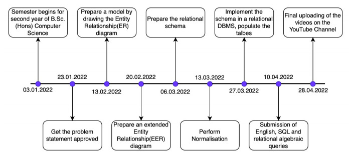
The purpose of the present research was to study the efficacy of learner-generated videos published on YouTube as a formative assessment method. The impact of the assessment method on students' learning and satisfaction, peer learning, group dynamics and skill development was analyzed. An emerging innovation within assessment was done with the students of an undergraduate computer science course during the COVID pandemic. Fifty-four students (teams of three to four) were instructed to create YouTube videos explaining the database design of a case study, peer-reviewed by views and likes. A mixed-method approach with a sequential study design was employed. A questionnaire with 25 questions on learners' and groups' attributes and four open-ended questions was administered. This was followed by a semi-structured interview comprising 19 questions. The quota sampling method was used for selecting a sample of students for interviews. Content analysis of interview transcripts was performed with the NVivo software.
During the experiment, we faced a challenge due to a lack of confidence among some students in public speaking. However, the innovative and engaging assessment resulted in the active participation of learners. Development of new skills like communication, peer bonding, teamwork and resolving conflicts was observed. Additionally, a fair and transparent grading methodology was a satisfying experience. Subject learning and video editing knowledge were enriched by peer learning. The results of the study revealed that publishing learner-generated videos on YouTube had a positive impact on students' learning and satisfaction. We therefore recommend the same as an effective tool for formative assessment.
Citation: Shikha Gupta, Sarika Tomar, Anamika Gupta. Learner-generated YouTube presentations for formative assessment[J]. STEM Education, 2023, 3(4): 306-330. doi: 10.3934/steme.2023019
The purpose of the present research was to study the efficacy of learner-generated videos published on YouTube as a formative assessment method. The impact of the assessment method on students' learning and satisfaction, peer learning, group dynamics and skill development was analyzed. An emerging innovation within assessment was done with the students of an undergraduate computer science course during the COVID pandemic. Fifty-four students (teams of three to four) were instructed to create YouTube videos explaining the database design of a case study, peer-reviewed by views and likes. A mixed-method approach with a sequential study design was employed. A questionnaire with 25 questions on learners' and groups' attributes and four open-ended questions was administered. This was followed by a semi-structured interview comprising 19 questions. The quota sampling method was used for selecting a sample of students for interviews. Content analysis of interview transcripts was performed with the NVivo software.
During the experiment, we faced a challenge due to a lack of confidence among some students in public speaking. However, the innovative and engaging assessment resulted in the active participation of learners. Development of new skills like communication, peer bonding, teamwork and resolving conflicts was observed. Additionally, a fair and transparent grading methodology was a satisfying experience. Subject learning and video editing knowledge were enriched by peer learning. The results of the study revealed that publishing learner-generated videos on YouTube had a positive impact on students' learning and satisfaction. We therefore recommend the same as an effective tool for formative assessment.

| [1] | Neo, M. and Neo, K.T., Innovative teaching: Using multimedia in a problem-based learning environment. Educational Technology & Society, 2001, 4(4): 19–31. |
| [2] |
Hansch, A., Hillers, L., McConachie, K., Newman, C., Schildhauer, T. and Schmidt, P., Video and online learning: Critical reflections and findings from the field. SSRN Electronic Journal, 2015. https://doi.org/10.2139/ssrn.2577882 doi: 10.2139/ssrn.2577882

|
| [3] | Sirkemaa, S. and Varpelaide, H., Experiences from using video in learning process. In EDULEARN16 Proceedings, 2016,460–465. https://doi.org/10.21125/edulearn.2016.1087 |
| [4] |
Brame, C.J., Effective educational videos: Principles and guidelines for maximizing student learning from video content. cbe life sciences education. CBE life sciences education, 2016, 15(4), es6. https://doi.org/10.1187/cbe.16-03-0125 doi: 10.1187/cbe.16-03-0125
|
| [5] |
Jorm, C., Roberts, C., Gordon, C., Nisbet, G. and Roper, L., Time for university educators to embrace student videography. Cambridge Journal of Education, 2019, 49(6): 673–693. https://doi.org/10.1080/0305764X.2019.1590528 doi: 10.1080/0305764X.2019.1590528
|
| [6] |
Abbas, N. and Qassim, T., Investigating the effectiveness of youtube as a learning tool among efl students at baghdad university. Arab World English Journal, 2020. https://doi.org/10.31235/osf.io/myqde doi: 10.31235/osf.io/myqde
|
| [7] | Gedera, D. and Zalipour, A., Video pedagogy theory and practice: Theory and practice, Springer, 2021. https://doi.org/10.1007/978-981-33-4009-1 |
| [8] |
Noetel, M., Griffith, S., Delaney, O., Sanders, T., Parker, P., del Pozo Cruz, B., et al., Video improves learning in higher education: A systematic review. Review of Educational Research, 2021, 91(2): 204–236. https://doi.org/10.3102/0034654321990713 doi: 10.3102/0034654321990713
|
| [9] | Berk, R., Multimedia teaching with video clips: Tv, movies, youtube, and mtvu in the college classroom. International Journal of Technology in Teaching and Learning, 2009, 5: 1–21. |
| [10] |
Azer, S., Algrain, H., Alkhelaif, R. and Aleshaiwi, S., Evaluation of the educational value of youtube videos about physical examination of the cardiovascular and respiratory systems. Journal of medical Internet research, 2013, 15(11): e2728. https://doi.org/10.2196/jmir.2728 doi: 10.2196/jmir.2728
|
| [11] |
DeWitt, D., Alias, N., Siraj, S., Yusaini, M., Ayob, J. and Ishak, R., The potential of youtube for teaching and learning in the performing arts. Procedia - Social and Behavioral Sciences, 2013,103: 1118–1126. https://doi.org/10.1016/j.sbspro.2013.10.439 doi: 10.1016/j.sbspro.2013.10.439
|
| [12] |
Sari, A., Dardjito, H. and Azizah, D., Efl students' improvement through the reflective youtube video project. International Journal of Instruction, 2020, 13(4): 393–408. https://doi.org/10.29333/iji.2020.13425a doi: 10.29333/iji.2020.13425a
|
| [13] |
Sedigheh, M., Ainin, S., Noor, I.J. and Nafisa, K., Social media as a complementary learning tool for teaching and learning: The case of youtube. The International Journal of Management Education, 2018, 16(1): 37–42. https://doi.org/10.1016/j.ijme.2017.12.001 doi: 10.1016/j.ijme.2017.12.001
|
| [14] |
Kaplan, A. and Haenlein, M., Users of the world, unite! the challenges and opportunities of social media. Business Horizons, 2010, 53(1): 59–68. https://doi.org/10.1016/j.bushor.2009.09.003 doi: 10.1016/j.bushor.2009.09.003
|
| [15] |
Greenhow, C., Robelia, B. and Hughes, J., Learning, teaching, and scholarship in a digital age: Web 2.0 and classroom research–what path should we take "now"? Educational Researcher, 2009, 38(4): 246–259. https://doi.org/10.3102/0013189X09336671 doi: 10.3102/0013189X09336671
|
| [16] | Harris, A. and Rea, A., Web 2.0 and virtual world technologies: A growing impact on is education. Journal of Information Systems Education, 2009, 20(2): 137–144. |
| [17] |
Epps, B., Luo, T. and Muljana, P., Lights, camera, activity! a systematic review of research on learner-generated videos. Journal of Information Technology Education: Research, 2021, 20: 405–427. https://doi.org/10.28945/4874 doi: 10.28945/4874
|
| [18] |
El-Said, O. and Aziz, H., Virtual tours a means to an end: An analysis of virtual tours' role in tourism recovery post covid-19. Journal of Travel Research, 2022, 61(3): 528–548. https://doi.org/10.1177/0047287521997567 doi: 10.1177/0047287521997567
|
| [19] |
Gallardo-Williams, M., Morsch, L., Paye, C. and Seery, M., Student-generated video in chemistry education. Chemistry Education Research and Practice, 2020, 21(2): 488–495. https://doi.org/10.1039/C9RP00182D doi: 10.1039/C9RP00182D
|
| [20] |
Pereira, J., Echeazarra, L., Sanz-Santamaría, S. and Gutiérrez, J., Student-generated online videos to develop cross-curricular and curricular competencies in nursing studies. Computers in Human Behavior, 2014, 31: 580–590. https://doi.org/10.1016/j.chb.2013.06.011 doi: 10.1016/j.chb.2013.06.011
|
| [21] |
Orús, C., Barlés, M.J., Belanche, D., Casaló, L., Fraj, E. and Gurrea, R., The effects of learner-generated videos for youtube on learning outcomes and satisfaction. Computers & Education, 2016, 95: 254–269. https://doi.org/10.1016/j.compedu.2016.01.007 doi: 10.1016/j.compedu.2016.01.007
|
| [22] | Reyna, J., Horgan, F., Ramp, D. and Meier, P., Using learner-generated digital media (lgdm) as an assessment tool in geological sciences. In 11th International Conference on Technology, Education and Development (INTED). Iated-int Assoc Technology Education & Development, 2017. https://doi.org/10.21125/inted.2017.0116 |
| [23] |
Reyna, J. and Meier, P., Using the learner-generated digital media (lgdm) framework in tertiary science education: A pilot study. Education Sciences, 2018, 8(3): 106. https://doi.org/10.3390/educsci8030106 doi: 10.3390/educsci8030106
|
| [24] |
Reyna, J., Digital media assignments in undergraduate science education: an evidence-based approach. Research in Learning Technology, 2021, 29. https://doi.org/10.25304/rlt.v29.2573 doi: 10.25304/rlt.v29.2573
|
| [25] |
Reyna, J. and Meier, P., Co-creation of knowledge using mobile technologies and digital media as pedagogical devices in undergraduate stem education. Research in Learning Technology, 2020, 28: 2356. https://doi.org/10.25304/rlt.v28.2356 doi: 10.25304/rlt.v28.2356
|
| [26] |
Belanche, D., Casaló, L.V., Orús, C. and Pérez-Rueda, A., Developing a learning network on youtube: Analysis of student satisfaction with a learner-generated content activity. Educational Networking: A Novel Discipline for Improved Learning Based on Social Networks, 2020,195–231. https://doi.org/10.1007/978-3-030-29973-6_6 doi: 10.1007/978-3-030-29973-6_6
|
| [27] |
Nikolic, S., Stirling, D. and Ros, M., Formative assessment to develop oral communication competency using youtube: self- and peer assessment in engineering. European Journal of Engineering Education, 2017, 43(4): 538–551. https://doi.org/10.1080/03043797.2017.1298569 doi: 10.1080/03043797.2017.1298569
|
| [28] | Zeballos, J., Meier, P. and Rodgers, K., Implementing digital media presentations as assessment tools for pharmacology students. American Journal of Educational Research, 2016, 4: 983–991. |
| [29] |
Fralinger, B. and Owens, R., You tube as a learning tool. Journal of College Teaching & Learning (TLC), 2009, 6(8). https://doi.org/10.19030/tlc.v6i8.1110 doi: 10.19030/tlc.v6i8.1110
|
| [30] | Pérez-Mateo, M., Maina, M.F., Guitert, M. and Romero, M., Learner generated content: Quality criteria in online collaborative learning. European Journal of Open, Distance and E-learning, 2011, 14(2). |
| [31] |
Podsakoff, P.M., MacKenzie, S.B., Lee, J.Y. and Podsakoff, N.P., Common method biases in behavioral research: a critical review of the literature and recommended remedies. Journal of applied psychology, 2003, 88(5): 879. https://doi.org/10.1037/0021-9010.88.5.879 doi: 10.1037/0021-9010.88.5.879
|


Figures(6) / Tables(1)
Shikha Gupta, Sarika Tomar, Anamika Gupta. Learner-generated YouTube presentations for formative assessment[J]. STEM Education, 2023, 3(4): 306-330. doi: 10.3934/steme.2023019


 DownLoad: