Continuous subsonic-sonic flows in a two-dimensional semi-infinitely long nozzle

Mingjun Zhou; Jingxue Yin; Mingjun Zhou; Jingxue Yin

doi:10.3934/era.2020122

Electronic Research Archive

2021, Volume 29, Issue 3: 2417-2444. doi: 10.3934/era.2020122

Previous Article Next Article

Special Issues

Continuous subsonic-sonic flows in a two-dimensional semi-infinitely long nozzle

Mingjun Zhou ^{1
,
,},
Jingxue Yin ^{2
,}

1.
School of Mathematics, Jilin University, Changchun 130012, China
2.
School of Mathematical Sciences, South China Normal University, Guangzhou 510631, China

Received: 01 August 2020 Revised: 01 October 2020 Published: 24 November 2020
35R35, 35Q35, 76N10, 35J70

This paper focuses on two-dimensional continuous subsonic-sonic potential flows in a semi-infinitely long nozzle with a straight lower wall and an upper wall which is convergent at the outlet while straight at the far fields. It is proved that if the variation rate of the cross section of the nozzle is suitably small, there exists a unique continuous subsonic-sonic flows in the nozzle such that the sonic curve intersects the upper wall at a fixed point and the velocity of the flow is along the normal direction at the sonic curve. Furthermore, the sonic curve is free, where the flow is singular in the sense that the flow speed is only Hölder continuous and the flow acceleration blows up. Additionally, the asymptotic behaviors of the flow speed at the far fields is shown.
- Degeneracy,
- free boundary,
- continuous subsonic-sonic flow,
- nonlocal boundary condition
Citation: Mingjun Zhou, Jingxue Yin. Continuous subsonic-sonic flows in a two-dimensional semi-infinitely long nozzle[J]. Electronic Research Archive, 2021, 29(3): 2417-2444. doi: 10.3934/era.2020122

Related Papers:

Abstract

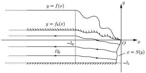
This paper focuses on two-dimensional continuous subsonic-sonic potential flows in a semi-infinitely long nozzle with a straight lower wall and an upper wall which is convergent at the outlet while straight at the far fields. It is proved that if the variation rate of the cross section of the nozzle is suitably small, there exists a unique continuous subsonic-sonic flows in the nozzle such that the sonic curve intersects the upper wall at a fixed point and the velocity of the flow is along the normal direction at the sonic curve. Furthermore, the sonic curve is free, where the flow is singular in the sense that the flow speed is only Hölder continuous and the flow acceleration blows up. Additionally, the asymptotic behaviors of the flow speed at the far fields is shown.

References

[1]	Existence and uniqueness of a subsonic flow past a given profile. Comm. Pure Appl. Math. (1954) 7: 441-504.
[2]	L. Bers, Mathematical Aspects of Subsonic and Transonic Gas Dynamics, John Wiley & Sons, Inc., New York; Chapman & Hall, Ltd., London, 1958.
[3]	On two-dimensional sonic-subsonic flow. Comm. Math. Phys. (2007) 271: 635-647.
[4]	Two dimensional subsonic Euler flows past a wall or a symmetric body. Arch. Ration. Mech. Anal. (2016) 221: 559-602.
[5]	Subsonic-sonic limit of approximate solutions to multidimensional steady Euler equations. Arch. Ration. Mech. Anal. (2016) 219: 719-740.
[6]	Steady Euler flows with large vorticity and characteristic discontinuities in arbitrary infinitely long nozzles. Adv. Math. (2019) 346: 946-1008.
[7]	Existence of steady subsonic Euler flows through infinitely long periodic nozzles. J. Differential Equations (2012) 252: 4315-4331.
[8]	R. Courant and K. O. Friedrichs, Supersonic Flow and Shock Waves, Interscience Publishers, Inc., New York, N. Y., 1948.
[9]	G. Dong, Nonlinear Partial Differential Equations of Second Order, Translations of Mathematical Monographs. 95, American Mathematical Society, Providence, RI, 1991. doi: 10.1090/mmono/095
[10]	Subsonic Euler flows with large vorticity through an infinitely long axisymmetric nozzle. J. Math. Fluid Mech. (2016) 18: 511-530.
[11]	Steady subsonic ideal flows through an infinitely long nozzle with large vorticity. Comm. Math. Phys. (2014) 328: 327-354.
[12]	Subsonic flows in a multi-dimensional nozzle. Arch. Ration. Mech. Anal. (2011) 201: 965-1012.
[13]	Three-dimensional subsonic flows, and asymptotic estimates for elliptic partial differential equations. Acta Math. (1957) 98: 265-296.
[14]	On multi-dimensional sonic-subsonic flow. Acta Math. Sci. Ser. B (Engl. Ed.) (2011) 31: 2131-2140.
[15]	A. Kuz'min, Boundary Value Problems for Transonic Flow, John Wiley and Sons, Ltd, 2002.
[16]	Continuous subsonic-sonic flows in convergent nozzles with straight solid walls. Nonlinearity (2016) 29: 86-130.
[17]	Continuous subsonic-sonic flows in a convergent nozzle. Acta Math. Sin. (Engl. Ser.) (2018) 34: 749-772.
[18]	Continuous subsonic-sonic flows in a general nozzle. J. Differential Equations (2015) 259: 2546-2575.
[19]	A free boundary problem of a degenerate elliptic equation and subsonic-sonic flows with general sonic curves. SIAM J. Math. Anal. (2019) 51: 4977-5010.
[20]	On a degenerate free boundary problem and continuous subsonic-sonic flows in a convergent nozzle. Arch. Ration. Mech. Anal. (2013) 208: 911-975.
[21]	A degenerate elliptic problem from subsonic-sonic flows in general nozzles. J. Differential Equations (2019) 267: 3778-3796.
[22]	Global subsonic and subsonic-sonic flows through infinitely long nozzles. Indiana Univ. Math. J. (2007) 56: 2991-3023.
[23]	Existence of global steady subsonic Euler flows through infinitely long nozzles. SIAM J. Math. Anal. (2010) 42: 751-784.
[24]	Global subsonic and subsonic-sonic flows through infinitely long axially symmetric nozzles. J. Differential Equations (2010) 248: 2657-2683.

Reader Comments

Your name:*

Email:*
© 2021 the Author(s), licensee AIMS Press. This is an open access article distributed under the terms of the Creative Commons Attribution License (http://creativecommons.org/licenses/by/4.0)