Retinal tears (RTs) are usually detected by B-scan ultrasound images, particularly for individuals with complex eye conditions. However, traditional manual techniques for reading ultrasound images have the potential to overlook or inaccurately diagnose conditions. Thus, the development of rapid and accurate approaches for the diagnosis of an RT is highly important and urgent. The present study introduces a novel hybrid deep-learning model called DCT-Net to enable the automatic and precise diagnosis of RTs. The implemented model utilizes a vision transformer as the backbone and feature extractor. Additionally, in order to accommodate the edge characteristics of the lesion areas, a novel module called the residual deformable convolution has been incorporated. Furthermore, normalization is employed to mitigate the issue of overfitting and, a Softmax layer has been included to achieve the final classification following the acquisition of the global and local representations. The study was conducted by using both our proprietary dataset and a publicly available dataset. In addition, interpretability of the trained model was assessed by generating attention maps using the attention rollout approach. On the private dataset, the model demonstrated a high level of performance, with an accuracy of 97.78%, precision of 97.34%, recall rate of 97.13%, and an F1 score of 0.9682. On the other hand, the model developed by using the public funds image dataset demonstrated an accuracy of 83.82%, a sensitivity of 82.69% and a specificity of 82.40%. The findings, therefore present a novel framework for the diagnosis of RTs that is characterized by a high degree of efficiency, accuracy and interpretability. Accordingly, the technology exhibits considerable promise and has the potential to serve as a reliable tool for ophthalmologists.
Citation: Ke Li, Qiaolin Zhu, Jianzhang Wu, Juntao Ding, Bo Liu, Xixi Zhu, Shishi Lin, Wentao Yan, Wulan Li. DCT-Net: An effective method to diagnose retinal tears from B-scan ultrasound images[J]. Mathematical Biosciences and Engineering, 2024, 21(1): 1110-1124. doi: 10.3934/mbe.2024046
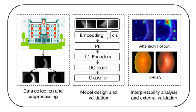
Retinal tears (RTs) are usually detected by B-scan ultrasound images, particularly for individuals with complex eye conditions. However, traditional manual techniques for reading ultrasound images have the potential to overlook or inaccurately diagnose conditions. Thus, the development of rapid and accurate approaches for the diagnosis of an RT is highly important and urgent. The present study introduces a novel hybrid deep-learning model called DCT-Net to enable the automatic and precise diagnosis of RTs. The implemented model utilizes a vision transformer as the backbone and feature extractor. Additionally, in order to accommodate the edge characteristics of the lesion areas, a novel module called the residual deformable convolution has been incorporated. Furthermore, normalization is employed to mitigate the issue of overfitting and, a Softmax layer has been included to achieve the final classification following the acquisition of the global and local representations. The study was conducted by using both our proprietary dataset and a publicly available dataset. In addition, interpretability of the trained model was assessed by generating attention maps using the attention rollout approach. On the private dataset, the model demonstrated a high level of performance, with an accuracy of 97.78%, precision of 97.34%, recall rate of 97.13%, and an F1 score of 0.9682. On the other hand, the model developed by using the public funds image dataset demonstrated an accuracy of 83.82%, a sensitivity of 82.69% and a specificity of 82.40%. The findings, therefore present a novel framework for the diagnosis of RTs that is characterized by a high degree of efficiency, accuracy and interpretability. Accordingly, the technology exhibits considerable promise and has the potential to serve as a reliable tool for ophthalmologists.

| [1] |
N. E. Byer, Natural history of posterior vitreous detachment with early management as the premier line of defense against retinal detachment, Ophthalmology, 101 (1994), 1503–1513. https://doi.org/10.1016/s0161-6420(94)31141-9 doi: 10.1016/s0161-6420(94)31141-9

|
| [2] |
J. Lorenzo-Carrero, I. Perez-Flores, M. Cid-Galano, M. Fernandez-Fernandez, F. Heras-Raposo, R. Vazquez-Nuñez, et al., B-scan ultrasonography to screen for retinal tears in acute symptomatic age-related posterior vitreous detachment, Ophthalmology, 116 (2009), 94–99. https://doi.org/10.1016/j.ophtha.2008.08.040 doi: 10.1016/j.ophtha.2008.08.040
|
| [3] |
J. AMDUR, A method of indirect ophthalmoscopy, Am. J. Ophthalmol., 48 (1959), 257–258. https://doi.org/10.1016/0002-9394(59)91247-4 doi: 10.1016/0002-9394(59)91247-4
|
| [4] |
K. E. Yong, Enhanced depth imaging optical coherence tomography of choroidal nevus: Comparison to B-Scan ultrasonography, J. Korean Ophthalmol. Soc., 55 (2014), 387–390. https://doi.org/10.3341/jkos.2014.55.3.387 doi: 10.3341/jkos.2014.55.3.387
|
| [5] |
M. S. Blumenkranz, S. F. Byrne, Standardized echography (ultrasonography) for the detection and characterization of retinal detachment, Ophthalmology, 89 (1982), 821–831. https://doi.org/10.1016/S0161-6420(82)34716-8 doi: 10.1016/S0161-6420(82)34716-8
|
| [6] |
H. C. Shin, H. R. Roth, M. Gao, L. Lu, Z. Xu, I. Nogues, et al., Deep convolutional neural networks for Computer-Aided detection: CNN architectures, dataset characteristics and transfer learning. IEEE Trans. Med. Imaging, 35 (2016), 1285–1298. https://doi.org/10.1109/TMI.2016.2528162 doi: 10.1109/TMI.2016.2528162
|
| [7] |
M. Chiang, D. Guth, A. A. Pardeshi, J. Randhawa, A. Shen, M. Shan, et al., Glaucoma expert-level detection of angle closure in goniophotographs with convolutional neural networks: the Chinese American eye study: Automated angle closure detection in goniophotographs, Am. J. Ophthalmol., 226 (2021), 100–107. https://doi.org/10.1016/j.ajo.2021.02.004 doi: 10.1016/j.ajo.2021.02.004
|
| [8] |
Z. Li, C. Guo, D. Lin, Y. Zhu, C. Chen, L. Zhang, et al., A deep learning system for identifying lattice degeneration and retinal breaks using ultra-widefield fundus images, Ann. Transl. Med., 7 (2019), 618. https://doi.org/10.21037/atm.2019.11.28 doi: 10.21037/atm.2019.11.28
|
| [9] |
C. Zhang, F. He, B. Li, H. Wang, X. He, X. Li, et al., Development of a deep-learning system for detection of lattice degeneration, retinal breaks, and retinal detachment in tessellated eyes using ultra-wide-field fundus images: a pilot study, Graefes Arch. Clin. Exp. Ophthalmol., 259 (2021), 2225–2234. https://doi.org/10.1007/s00417-021-05105-3 doi: 10.1007/s00417-021-05105-3
|
| [10] | A. Dosovitskiy, L. Beyer, A. Kolesnikov, D. Weissenborn, X. Zhai, T. Unterthiner, et al., An image is worth 16x16 words: Transformers for image recognition at scale, preprint, arXiv: 2010.11929. |
| [11] | A. Vaswani, N. Shazeer, N. Parmar, J. Uszkoreit, L. Jones, A. N. Gomez, et al., Attention is all you need, preprint, arXiv: 1706.03762. |
| [12] |
Z. Jiang, L. Wang, Q. Wu, Y. Shao, M. Shen, W. Jiang, et al., Computer-aided diagnosis of retinopathy based on vision transformer, J. Innov. Opt. Health Sci., 15 (2022), 2250009. https://doi.org/10.1142/S1793545822500092 doi: 10.1142/S1793545822500092
|
| [13] |
J. Wu, R. Hu, Z. Xiao, J. Chen, J. Liu, Vision Transformer-based recognition of diabetic retinopathy grade, Med. Phys., 48 (2021), 7850–7863. https://doi.org/10.1002/mp.15312 doi: 10.1002/mp.15312
|
| [14] | J. Dai, H. Qi, Y. Xiong, Y. Li, G. Zhang, H. Hu, et al., Deformable convolutional networks, preprint, arXiv: 1703.06211. |
| [15] | P. T. Jackson, A. A. Abarghouei, S. Bonner, T. P. Breckon, B. Obara, Style augmentation: data augmentation via style randomization, CVPR Workshops, 6 (2019), 10–11. |
| [16] | Z. Zhong, L. Zheng, G. Kang, S. Li, Y. Yang, Random erasing data augmentation, in Proceedings of the AAAI conference on artificial intelligence, 34 (2020), 13001–13008. |
| [17] | C. Bowles, L. Chen, R. Guerrero, P. Bentley, R. Gunn, A. Hammers, et al., Gan augmentation: Augmenting training data using generative adversarial networks, preprint, arXiv: 1810.10863. |
| [18] | J. Devlin, M. W. Chang, K. Lee, K. Toutanova, Bert: Pre-training of deep bidirectional transformers for language understanding, in Proceedings of naacL-HLT, 1 (2019), 2. |
| [19] | K. He, X. Zhang, S. Ren, J. Sun, Deep residual learning for image recognition, in Proceedings of the IEEE conference on computer vision and pattern recognition, (2016), 770–778. |
| [20] |
S. Hochreiter, The vanishing gradient problem during learning recurrent neural nets and problem solutions, Int. J. Uncertainty Fuzziness Knowledge Based Syst., 6 (1998), 107–116. https://doi.org/10.1142/S0218488598000094 doi: 10.1142/S0218488598000094
|
| [21] | P. Murugan, S. Durairaj, Regularization and optimization strategies in deep convolutional neural network, preprint, arXiv: 1712.04711. |
| [22] | C. C. J. Kuo, M. Zhang, S. Li, J. Duan, Y. Chen, Interpretable convolutional neural networks via feedforward design, preprint, arXiv: 1810.02786. |
| [23] | Z. Zhang, H. Zhang, L. Zhao, T. Chen, S. Ö. Arik, T. Pfister, Nested hierarchical transformer: Towards accurate, data-efficient and interpretable visual understanding, preprint, arXiv: 2105.12723. |
| [24] | R. R. Selvaraju, M. Cogswell, A. Das, R. Vedantam, D. Parikh, D. Batra, Grad-CAM: Why did you say that? Visual explanations from deep networks via gradient-based localization, preprint, arXiv: 1610.02391. |
| [25] | S. Abnar, W. Zuidema, Quantifying attention flow in transformers, preprint, arXiv: 2005.00928. |
| [26] | M. C. Dickson, A. S. Bosman, K. M. Malan, Hybridised loss functions for improved neural network generalisation, preprint, arXiv: 2204.12244. |
| [27] | C. Ma, D. Kunin, L. Wu, L. Ying, Beyond the quadratic approximation: the multiscale structure of neural network loss landscapes, preprint, arXiv: 2204.11326. |
| [28] | S. J. Reddi, S. Kale, S. Kumar, On the convergence of adam and beyond, preprint, arXiv: 1904.09237. |
| [29] | A. Krizhevsky, I. Sutskever, G. E. Hinton, ImageNet classification with deep convolutional neural networks, Adv. Neural Inform. Process. Syst., 25 (2012), 2. |
| [30] | C. Szegedy, V. Vanhoucke, S. Ioffe, J. Shlens, Z. Wojna, Rethinking the inception architecture for computer vision, in Proceedings of the IEEE conference on computer vision and pattern recognition, (2016), 2818–2826. |
| [31] | K. Simonyan, A. Zisserman, Very deep convolutional networks for large-scale image recognition, preprint, arXiv: 1409.1556. |
| [32] | J. Lorenzo-Carrero, I. Perez-Flores, M. Cid-Galano, M. Fernandez-Fernandez, F. Heras-Raposo, R. Vazquez-Nuñez, et al., B-scan ultrasonography to screen for retinal tears in acute symptomatic age-related posterior vitreous detachment, Ophthalmology, 116 (2009), 94–99. https://doi.org/1016/j.ophtha.2008.08.040 |
| [33] |
X. Xu, Y. Guan, J. Li, Z. Ma, L. Zhang, L. Li, Automatic glaucoma detection based on transfer induced attention network, Biomed. Eng. Online, 20 (2021), 1–19. https://doi.org/10.1186/s12938-021-00877-5 doi: 10.1186/s12938-021-00877-5
|
| [34] | X. Chen, Y. Xu, S. Yan, D. W. K. Wong, T. Y. Wong, J. Liu, Automatic feature learning for glaucoma detection based on deep learning, in Medical Image Computing and Computer-Assisted Intervention, 18 (2015). |
| [35] |
N. Shibata, M. Tanito, K. Mitsuhashi, Y. Fujino, M. Matsuura, H. Murata, et al., Development of a deep residual learning algorithm to screen for glaucoma from fundus photography, Sci. Rep., 8 (2018), 14665. https://doi.org/10.1038/s41598-018-33013-w doi: 10.1038/s41598-018-33013-w
|
| [36] |
Y. Yu, M. Rashidi, B. Samali, M. Mohammadi, T. N. Nguyen, X. Zhou, Crack detection of concrete structures using deep convolutional neural networks optimized by enhanced chicken swarm algorithm, Struct. Health Monit., 5 (2022), 2244–2263. https://doi.org/10.1177/14759217211053546 doi: 10.1177/14759217211053546
|
| [37] |
Y. Yu, B. Samali, M. Rashidi, M. Mohammadi, T. N. Nguyen, G. Zhang, Vision-based concrete crack detection using a hybrid framework considering noise effect, J. Build Eng., 61 (2022), 105246. https://doi.org/10.1016/j.jobe.2022.105246 doi: 10.1016/j.jobe.2022.105246
|
| [38] |
B. Ragupathy, M. Karunakaran, A fuzzy logic‐based meningioma tumor detection in magnetic resonance brain images using CANFIS and U-Net CNN classification, Int. J. Imaging Syst. Technol., 31(2021), 379–390. https://doi.org/10.1002/ima.22464 doi: 10.1002/ima.22464
|
| [39] |
Z. Jiang, L. Wang, Q. Wu, Y. Shao, M. Shen, W. Jiang, et al., Computer-aided diagnosis of retinopathy based on vision transformer, J. Innov. Opt. Health Sci., 15 (2022), 2250009. https://doi.org/10.1142/S1793545822500092 doi: 10.1142/S1793545822500092
|


Figures(6) / Tables(3)

Ke Li, Qiaolin Zhu, Jianzhang Wu, Juntao Ding, Bo Liu, Xixi Zhu, Shishi Lin, Wentao Yan, Wulan Li. DCT-Net: An effective method to diagnose retinal tears from B-scan ultrasound images[J]. Mathematical Biosciences and Engineering, 2024, 21(1): 1110-1124. doi: 10.3934/mbe.2024046


 DownLoad: