A novel attention-guided ECA-CNN architecture for sEMG-based gait classification

Zhangjie Wu; Minming Gu; Zhangjie Wu; Minming Gu

doi:10.3934/mbe.2023308

Mathematical Biosciences and Engineering

2023, Volume 20, Issue 4: 7140-7153. doi: 10.3934/mbe.2023308

Previous Article Next Article

Research article Special Issues

A novel attention-guided ECA-CNN architecture for sEMG-based gait classification

Zhangjie Wu ,
Minming Gu ^,

School of Information Science and Technology, Zhejiang Sci-Tech University, Hangzhou 310018, China

Academic Editor: Yang Kuang

Received: 08 November 2022 Revised: 12 January 2023 Accepted: 01 February 2023 Published: 10 February 2023

Gait recognition and classification technology is one of the essential technologies for detecting neurodegenerative dysfunction. This paper presents a gait classification model based on a convolutional neural network (CNN) with an efficient channel attention (ECA) module for gait detection applications using surface electromyographic (sEMG) signals. First, the sEMG sensor was used to collect the experimental sample data, and various gaits of different persons were collected to construct the sEMG signal data sets of different gaits. The CNN is used to extract the features of the one-dimensional input sEMG signal to obtain the feature vector, which is input into the ECA module to realize cross-channel interaction. Then, the next part of the convolutional layer is input to learn the signal features further. Finally, the model is output and tested to obtain the results. Comparative experiments show that the accuracy of the ECA-CNN network model can reach 97.75%.
- surface electromyography,
- convolutional neural networks,
- efficient channel attention mechanism,
- gait classification,
- neurodegenerative disease prevention
Citation: Zhangjie Wu, Minming Gu. A novel attention-guided ECA-CNN architecture for sEMG-based gait classification[J]. Mathematical Biosciences and Engineering, 2023, 20(4): 7140-7153. doi: 10.3934/mbe.2023308

Related Papers:

Abstract

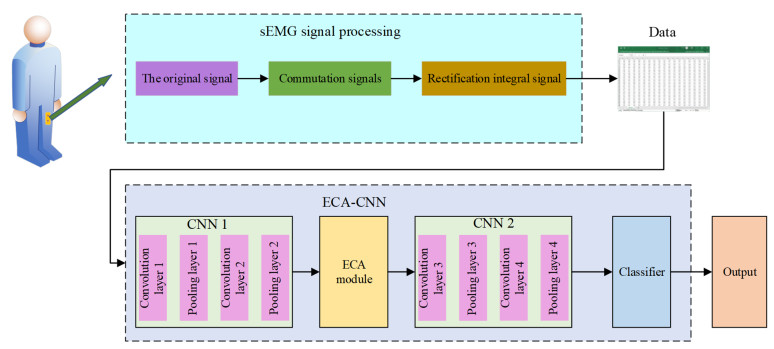
Gait recognition and classification technology is one of the essential technologies for detecting neurodegenerative dysfunction. This paper presents a gait classification model based on a convolutional neural network (CNN) with an efficient channel attention (ECA) module for gait detection applications using surface electromyographic (sEMG) signals. First, the sEMG sensor was used to collect the experimental sample data, and various gaits of different persons were collected to construct the sEMG signal data sets of different gaits. The CNN is used to extract the features of the one-dimensional input sEMG signal to obtain the feature vector, which is input into the ECA module to realize cross-channel interaction. Then, the next part of the convolutional layer is input to learn the signal features further. Finally, the model is output and tested to obtain the results. Comparative experiments show that the accuracy of the ECA-CNN network model can reach 97.75%.

References

[1]	A. Gulland, Global life expectancy has risen, reports WHO, BMJ, 348 (2014). https://doi.org/10.1136/bmj.g3369 doi: 10.1136/bmj.g3369
[2]	W. C. Sanderson, S. Scherbov, The Characteristics approach to the measurement of population aging, Popul. Dev. Rev., 39 (2013), 673–685. https://doi.org/10.1111/j.1728-4457.2013.00633.x doi: 10.1111/j.1728-4457.2013.00633.x
[3]	A. Snijders, N. Giladi, B. Bloem, B. van de Warrenburg, Neurological gait disorders in elderly people: clinical approach and classification, Lancet Neurol., 6 (2007), 63–74. https://doi.org/10.1016/S1474-4422(06)70678-0 doi: 10.1016/S1474-4422(06)70678-0
[4]	C. Artusi, M. Mishra, P. Latimer, J. Vizcarra, L. Lopiano, W. Maetzler, et al., Integration of technology-based outcome measures in clinical trials of Parkinson and other neurodegenerative diseases, Parkinsonism Relat. Disord., 46 (2018), 53–56. https://doi.org/10.1016/j.parkreldis.2017.07.022 doi: 10.1016/j.parkreldis.2017.07.022
[5]	J. Li, The experiences of early detection, early diagnosis and early treatment of cancer in rural areas of China, J. Global Oncol., 4 (2018). https://doi.org/10.1200/jgo.18.60300 doi: 10.1200/jgo.18.60300
[6]	G. Emayavaramban, S. Divyapriya, V. M. Mansoor, A. Amudha, M. Ramkumar, P. Nagaveni, et al., SEMG based classification of hand gestures using artificial neural network, Mater. Today Proc., 37 (2021), 2591–2598. https://doi.org/10.1016/j.matpr.2020.08.504 doi: 10.1016/j.matpr.2020.08.504
[7]	N. Karnam, A. Turlapaty, S. Dubey, B. Gokaraju, Classification of sEMG signals of hand gestures based on energy features, Biomed. Signal Process. Control, 70 (2021). https://doi.org/10.1016/J.BSPC.2021.102948 doi: 10.1016/J.BSPC.2021.102948
[8]	G. I. Papagiannis, A. I. Triantafyllou, I. M. Roumpelakis, F. Zampeli, P. Eleni, P. Koulouvaris, et al., Methodology of surface electromyographyin gait analysis: review of the literature, J. Med. Eng. Technol., 43 (2019), 59–65. https://doi.org/10.1080/03091902.2019.1609610 doi: 10.1080/03091902.2019.1609610
[9]	C. Frigo, P. Crenna, Multichannel SEMG in clinical gait analysis: A review and state-of-the-art, Clin. Biomech., 24 (2008), 236–245. https://doi.org/10.1016/j.clinbiomech.2008.07.012 doi: 10.1016/j.clinbiomech.2008.07.012
[10]	S. Cai, Y. Chen, S. Huang, Y. Wu, H. Zheng, X. Li, et al., SVM-Based classification of sEMG signals for upper-limb self-rehabilitation training, Front. Neurorob., 13 (2019). https://doi.org/10.3389/fnbot.2019.00031 doi: 10.3389/fnbot.2019.00031
[11]	J. Miller, M. Beazer, M. Hahn, Myoelectric walking mode classification for transtibial amputees, IEEE Trans. Biomed. Eng., 60 (2013), 2745–2750 https://doi.org/10.1109/TBME.2013.2264466 doi: 10.1109/TBME.2013.2264466
[12]	G. R. Naik, S. Selvan, S. Arjunan, A. Acharyya, D. Kumar, A. Ramanujam, et al., An ICA-EBM-based sEMG classifier for recognizing lower limb movements in individuals with and without knee pathology, IEEE Trans. Neural Syst. Rehabil. Eng., 26 (2018), 675–686. https://doi.org/10.1109/TNSRE.2018.2796070 doi: 10.1109/TNSRE.2018.2796070
[13]	Y. Narayan, SEMG signal classification using KNN classifier with FD and TFD features, Mater. Today Proc., 37 (2021), 3219–3225. https://doi.org/10.1016/j.matpr.2020.09.089 doi: 10.1016/j.matpr.2020.09.089
[14]	R. Jaehwan, B. Lee, J. Maeng, D. Kim, sEMG-signal and IMU sensor-based gait sub-phase detection and prediction using a user-adaptive classifier, Med. Eng. Phys., 69 (2019), 50–57. https://doi.org/10.1016/j.medengphy.2019.05.006 doi: 10.1016/j.medengphy.2019.05.006
[15]	P. Wei, J. Zhang, F. Tian, J. Hong, A comparison of neural networks algorithms for EEG and sEMG features based gait phases recognition, Biomed. Signal Process. Control, 68 (2021). https://doi.org/10.1016/j.bspc.2021.102587 doi: 10.1016/j.bspc.2021.102587
[16]	W. Piatkowska, F. Spolaor, M. Romanato, R. Polli, A. Huang, A. Murgia, et al., A supervised classification of children with fragile X syndrome and controls based on kinematic and sEMG parameters, Appl. Sci., 12 (2022), 1612. https://doi.org/10.3390/app12031612 doi: 10.3390/app12031612
[17]	X. Zhang, S. Sun, C. Li, Z. Tang, Impact of load variation on the accuracy of gait recognition from surface EMG signals, Appl. Sci., 8 (2018), 1462. https://doi.org/10.3390/app8091462 doi: 10.3390/app8091462
[18]	M. Meng, Q. She, Y. Gao, Z. Luo, EMG signals based gait phases recognition using hidden Markov models, in The 2010 IEEE International Conference on Information and Automation, (2010), 852–856. https://doi.org/10.1109/ICINFA.2010.5512456.
[19]	H. Zhao, Z. Wang, S. Qiu, J. Wang, F. Xu, Z. Wang, et al., Adaptive gait detection based on foot-mounted inertial sensors and multi-sensor fusion, Inf. Fusion, 52 (2019), 157–166. https://doi.org/10.1016/j.inffus.2019.03.002 doi: 10.1016/j.inffus.2019.03.002
[20]	D. Xiong, D. Zhang, X. Zhao, Y. Chu, Y. Zhao, Synergy-based neural interface for human gait tracking with deep learning, IEEE Trans. Neural Syst. Rehabil. Eng., 29 (2021), 2271–2280. https://doi.org/10.1109/TNSRE.2021.3123630. doi: 10.1109/TNSRE.2021.3123630
[21]	A. Vijayvargiya, Khimraj, R. Kumar, N. Dey, Voting-based 1D CNN model for human lower limb activity recognition using sEMG signal, Phys. Eng. Sci. Med., 44 (2021), 1297–1309. https://doi.org/10.1007/s13246-021-01071-6 doi: 10.1007/s13246-021-01071-6
[22]	M. Coskun, O. Yildirim, Y. Demir, U. Acharya, Efficient deep neural network model for classification of grasp types using sEMG signals, J. Ambient Intell. Hum. Comput., 13 (2022), 4437–4450. https://doi.org/10.1007/s12652-021-03284-9 doi: 10.1007/s12652-021-03284-9
[23]	Q. Ni, M. Zhang, STGMN: A gated multi-graph convolutional network framework for traffic flow prediction, Appl. Intell., 52 (2022), 15026–15039. https://doi.org/10.1007/s10489-022-03224-w doi: 10.1007/s10489-022-03224-w
[24]	J. Shen, Z. Zheng, Y. Sun, M. Zhao, Y. Chang, Y. Shao, et al., HAMNet: hyperspectral image classification based on hybrid neural network with attention mechanism and multi-scale feature fusion, Int. J. Remote Sens., 43 (2022), 4233–4258. https://doi.org/10.1080/01431161.2022.2109222 doi: 10.1080/01431161.2022.2109222
[25]	A. Vijayvargiya, B. Singh, R. Kumar, J. Tavares, Human lower limb activity recognition techniques, databases, challenges and its applications using sEMG signal: an overview, Biomed. Eng. Lett., 12 (2022), 343–358. https://doi.org/10.1007/s13534-022-00236-w doi: 10.1007/s13534-022-00236-w
[26]	D. Yungher, M. Wininger, J. Barr, W. Craelius, A. Threlkeld, Surface muscle pressure as a measure of active and passive behavior of muscles during gait, Med. Eng. Phys., 33 (2011), 464–471. https://doi.org/10.1016/j.medengphy.2010.11.012 doi: 10.1016/j.medengphy.2010.11.012
[27]	H. Sun, L. Wang, R. Lin, Z. Zhang, B. Zhang, Mapping plastic greenhouses with two-temporal sentinel-2 images and 1D-CNN deep learning, Remote Sens., 13 (2021). https://doi.org/10.3390/rs13142820 doi: 10.3390/rs13142820
[28]	B. Whittington, A. Silder, B. Heiderscheit, D. G. Thelen, The contribution of passive-elastic mechanisms to lower extremity joint kinetics during human walking, Gait Posture, 27 (2008), 628–634. https://doi.org/10.1016/j.gaitpost.2007.08.005 doi: 10.1016/j.gaitpost.2007.08.005
[29]	S. Liu, S. You, C. Zeng, H. Yin, Z. Lin, Y. Dong, et al., Data source authentication of synchrophasor measurement devices based on 1D-CNN and GRU, Electr. Power Syst. Res., 196 (2021). https://doi.org/10.1016/j.epsr.2021.107207 doi: 10.1016/j.epsr.2021.107207
[30]	Q. Wang, B. Wu, P. Zhu, P. Li, W. Zuo, Q. Hu, ECA-Net: Efficient channel attention for deep convolutional neural networks, in 2020 IEEE/CVF Conference on Computer Vision and Pattern Recognition (CVPR), (2020), 11531–11539. https://doi.org/10.1109/CVPR42600.2020.01155
[31]	T. Arakawa, T. Otani, Y. Kobayashi, M. Tanaka, 2-D forward dynamics simulation of gait adaptation to muscle weakness in elderly gait, Gait Posture, 85 (2021), 71–77. https://doi.org/10.1016/j.gaitpost.2021.01.011 doi: 10.1016/j.gaitpost.2021.01.011
[32]	G. Cicirelli, D. Impedovo, V. Dentamaro, R. Marani, G. Pirlo, T. R. D'Orazio, Human gait analysis in neurodegenerative diseases: a review, IEEE J. Biomed. Health Inf., 26 (2022), 229–242. https://doi.org/10.1109/JBHI.2021.3092875 doi: 10.1109/JBHI.2021.3092875
[33]	J. A. Martin, M. W. Kindig, C. J. Stender, W. R. Ledoux, D. G. Thelen, Calibration of the shear wave speed-stress relationship in in situ Achilles tendons using cadaveric simulations of gait and isometric contraction, J. Biomech., 106 (2020), 109799. https://doi.org/10.1016/j.jbiomech.2020.109799 doi: 10.1016/j.jbiomech.2020.109799
[34]	M. Woiczinski, C. Lehner, T. Esser, M. Kistler, M. Azqueta, J. Leukert, et al., Influence of treadmill design on gait: Does treadmill size affect muscle activation amplitude? A musculoskeletal calculation with individualized input parameters of gait analysis, Front. Neurol., 13 (2022), 830762–830762. https://doi.org/10.3389/fneur.2022.830762 doi: 10.3389/fneur.2022.830762

Reader Comments

Your name:*

Email:*
© 2023 the Author(s), licensee AIMS Press. This is an open access article distributed under the terms of the Creative Commons Attribution License (http://creativecommons.org/licenses/by/4.0)