Accurate cloud detection is an important step to improve the utilization rate of remote sensing (RS). However, existing cloud detection algorithms have difficulty in identifying edge clouds and broken clouds. Therefore, based on the channel data of the Himawari-8 satellite, this work proposes a method that combines the feature enhancement module with the Gaussian mixture model (GMM). First, statistical analysis using the probability density functions (PDFs) of spectral data from clouds and underlying surface pixels was conducted, selecting cluster features suitable for daytime and nighttime. Then, in this work, the Laplacian operator is introduced to enhance the spectral features of cloud edges and broken clouds. Additionally, enhanced spectral features are input into the debugged GMM model for cloud detection. Validation against visual interpretation shows promising consistency, with the proposed algorithm outperforming other methods such as RF, KNN and GMM in accuracy metrics, demonstrating its potential for high-precision cloud detection in RS images.
Citation: Fangrong Zhou, Gang Wen, Yi Ma, Yutang Ma, Hao Pan, Hao Geng, Jun Cao, Yitong Fu, Shunzhen Zhou, Kaizheng Wang. A two-branch cloud detection algorithm based on the fusion of a feature enhancement module and Gaussian mixture model[J]. Mathematical Biosciences and Engineering, 2023, 20(12): 21588-21610. doi: 10.3934/mbe.2023955
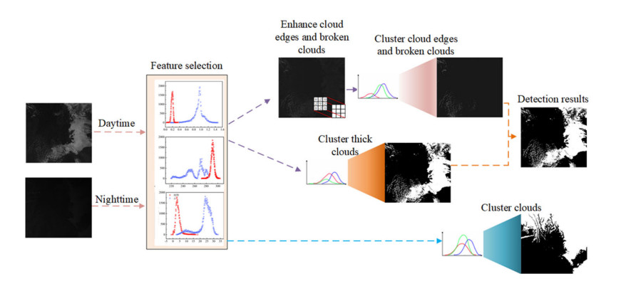
Accurate cloud detection is an important step to improve the utilization rate of remote sensing (RS). However, existing cloud detection algorithms have difficulty in identifying edge clouds and broken clouds. Therefore, based on the channel data of the Himawari-8 satellite, this work proposes a method that combines the feature enhancement module with the Gaussian mixture model (GMM). First, statistical analysis using the probability density functions (PDFs) of spectral data from clouds and underlying surface pixels was conducted, selecting cluster features suitable for daytime and nighttime. Then, in this work, the Laplacian operator is introduced to enhance the spectral features of cloud edges and broken clouds. Additionally, enhanced spectral features are input into the debugged GMM model for cloud detection. Validation against visual interpretation shows promising consistency, with the proposed algorithm outperforming other methods such as RF, KNN and GMM in accuracy metrics, demonstrating its potential for high-precision cloud detection in RS images.

| [1] |
I. Z. Cetin, H. Sevik, Investigation of the relationship between bioclimatic comfort and land use by using GIS and RS techniques in Trabzon, Environ. Monit. Assess., 192 (2020), 1–14. https://doi.org/10.1007/s10661-019-8029-4 doi: 10.1007/s10661-019-8029-4

|
| [2] |
K. Kak, Satellite remote sensing for disaster management support: A holistic and staged approach based on case studies in Sentinel Asia, Int. J. Disaster Risk Reduct., 33 (2019), 417–432. https://doi.org/10.1016/j.ijdrr.2018.09.015 doi: 10.1016/j.ijdrr.2018.09.015
|
| [3] |
P. Barmpoutis, P. Papaioannou, K. Dimitropoulos, N. Grammalidis, A review on early forest fire detection systems using optical remote sensing, Sensors, 20 (2020), 6442. https://doi.org/10.3390/s20226442 doi: 10.3390/s20226442
|
| [4] |
T. P. P. Sharma, J. Zhang, U. A. Koju, S. Zhang, Y. Bai, M. K. Suwal, Review of flood disaster studies in Nepal: A remote sensing perspective, J. Disaster Risk Reduct., 34 (2019), 18–27. https://doi.org/10.1016/j.ijdrr.2018.11.022 doi: 10.1016/j.ijdrr.2018.11.022
|
| [5] |
R. R. Girija, S. Mayappan, Mapping of mineral resources and lithological units: A review of remote sensing techniques, Int. J. Image Data Fusion., 10 (2019), 79–106. https://doi.org/10.1080/19479832.2019.1589585 doi: 10.1080/19479832.2019.1589585
|
| [6] |
G. L. Spadoni, A. Cavalli, L. Congedo, M. Munafò, Analysis of normalized difference vegetation index (NDVI) multi-temporal series for the production of forest cartography, Remote Sens. Appl., 20 (2020), 100419. https://doi.org/10.1016/j.rsase.2020.100419 doi: 10.1016/j.rsase.2020.100419
|
| [7] | H. Harde, How much CO2 and the sun contribute to global warming: Comparison of simulated temperature trends with last century observations, Sci. Clim. Change, 2 (2022), 105–133. |
| [8] |
Q. He, X. Sun, Z. Yan, K. Fu, DABNet: Deformable contextual and boundary-weighted network for cloud detection in remote sensing images, IEEE Trans. Geosci. Remote Sens., 60 (2021), 1–16. https://doi.org/10.1109/TGRS.2020.3045474 doi: 10.1109/TGRS.2020.3045474
|
| [9] |
W. Rossow, E. Duenas, The international satellite cloud climatology project (ISCCP) web site: An online resource for research, Bull. Am. Meteorol. Soc., 85 (2004), 167–172. https://doi.org/10.1175/BAMS-85-2-167 doi: 10.1175/BAMS-85-2-167
|
| [10] |
Q. Xiong, Y. Wang, D. Liu, S. Ye, Z. Du, W. Liu, et al., A cloud detection approach based on hybrid multispectral features with dynamic thresholds for GF-1 remote sensing images, Remote Sens., 12 (2020), 450. https://doi.org/10.3390/rs12030450 doi: 10.3390/rs12030450
|
| [11] |
P. Li, L. Dong, H. Xiao, M. Xu, A cloud image detection method based on SVM vector machine, Neurocomputing, 169 (2015), 34–42. https://doi.org/10.1016/j.neucom.2014.09.102 doi: 10.1016/j.neucom.2014.09.102
|
| [12] |
W. Zhang, S. Jin, L. Zhou, X. Xie, F. Wang, L. Jiang, et al., Multi-feature embedded learning SVM for cloud detection in remote sensing images, Comput. Electr. Eng., 102 (2022), 108177. https://doi.org/10.1016/j.compeleceng.2022.108177 doi: 10.1016/j.compeleceng.2022.108177
|
| [13] |
H. Ishida, Y. Oishi, K. Morita, K. Moriwaki, T. Y. Nakajima, Development of a support vector machine based cloud detection method for MODIS with the adjustability to various conditions, Remote Sens. Environ., 205 (2018), 390–407. https://doi.org/10.1016/j.rse.2017.11.003 doi: 10.1016/j.rse.2017.11.003
|
| [14] |
N. Ghasemian, M. Akhoondzadeh, Introducing two random forest based methods for cloud detection in remote sensing images, Adv. Space. Res., 62 (2018), 288–303. https://doi.org/10.1016/j.asr.2018.04.030 doi: 10.1016/j.asr.2018.04.030
|
| [15] |
H. Fu, Y. Shen, J. Liu, G. He, J. Chen, P. Liu, et al., Cloud detection for FY meteorology satellite based on ensemble thresholds and random forests approach, Remote Sens., 11 (2018), 44. https://doi.org/10.3390/rs11010044 doi: 10.3390/rs11010044
|
| [16] |
J. Zhang, J. Wu, H. Wang, Y. Wang, Y. Li, Cloud detection method using CNN based on cascaded feature attention and channel attention, IEEE Trans. Geosci. Remote Sens., 60 (2021), 1–17. https://doi.org/10.1109/TGRS.2021.3120752 doi: 10.1109/TGRS.2021.3120752
|
| [17] |
F. Xie, M. Shi, Z. Shi, J. Yin, D. Zhao, Multilevel cloud detection in remote sensing images based on deep learning, IEEE J. Sel. Top. Appl. Earth Obs. Remote Sens., 10 (2017), 3631–3640. https://doi.org/10.1109/JSTARS.2017.2686488 doi: 10.1109/JSTARS.2017.2686488
|
| [18] |
L. Sun, X. Yang, S. Jia, C. Jia, Q. Wang, X. Liu, et al., Satellite data cloud detection using deep learning supported by hyperspectral data, Int. J. Remote Sens., 41 (2020), 1349–1371. https://doi.org/10.1080/01431161.2019.1667548 doi: 10.1080/01431161.2019.1667548
|
| [19] |
D. A. Reynolds, Gaussian mixture models, Encycl. Biom., 741 (2009), 659–663. https://doi.org/10.1007/978-0-387-73003-5_196 doi: 10.1007/978-0-387-73003-5_196
|
| [20] |
D. Zhang, C. Huang, J. Gu, J. Hou, Y. Zhang, W. Han, et al., Real-time wildfire detection algorithm based on VⅡRS fire product and Himawari-8 data, Remote Sens., 15 (2023), 1541. https://doi.org/10.3390/rs15061541 doi: 10.3390/rs15061541
|
| [21] |
Y. Kang, T. Sung, J. Im, Toward an adaptable deep-learning model for satellite-based wildfire monitoring with consideration of environmental conditions, Remote Sens. Environ., 298 (2023), 113814. https://doi.org/10.1016/j.rse.2023.113814 doi: 10.1016/j.rse.2023.113814
|
| [22] |
J. Xia, N. Yokoya, B. Adriano, K. Kanemoto, National high-resolution cropland classification of Japan with agricultural census information and multi-temporal multi-modality datasets, Int. J. Appl. Earth Obs. Geoinf., 117 (2023), 103193. https://doi.org/10.1016/j.jag.2023.103193 doi: 10.1016/j.jag.2023.103193
|
| [23] |
X. Li, Y. Qu, H. Geng, Q. Xin, J. Huang, S. Peng, et al., Mapping annual 10-m maize cropland changes in China during 2017–2021, Sci. Data, 10 (2023), 765. https://doi.org/10.1038/s41597-023-02665-3 doi: 10.1038/s41597-023-02665-3
|
| [24] |
C. Huang, N. Thomas, S. N. Goward, J. G. Masek, Z. Zhu, R. G. John, Automated masking of cloud and cloud shadow for forest change analysis using Landsat images, Int. J. Remote Sens., 31 (2010), 5449–5464. https://doi.org/10.1080/01431160903369642 doi: 10.1080/01431160903369642
|
| [25] |
X. Long, X Li, H. Lin, M. Zhang, Mapping the vegetation distribution and dynamics of a wetland using adaptive-stacking and google earth engine based on multi-source remote sensing data, Int. J. Appl. Earth Obs. Geoinf., 102 (2021): 102453. https://doi.org/10.1016/j.jag.2021.102453 doi: 10.1016/j.jag.2021.102453
|
| [26] |
B. Chen, J. Hu, Z. Song, X. Zhou, L. Zhao, Y. Wang, et al., Exploring high-resolution near-surface CO concentrations based on Himawari-8 top-of-atmosphere radiation data: Assessing the distribution of city-level CO hotspots in China, Atmos. Environ., 312 (2023), 120021. https://doi.org/10.1016/j.atmosenv.2023.120021 doi: 10.1016/j.atmosenv.2023.120021
|
| [27] |
W. Xu, W. Wang, N. Wang, B. Chen, A new algorithm for Himawari-8 aerosol optical depth retrieval by integrating regional PM2.5 concentrations, IEEE Trans. Geosci. Remote Sens., 60 (2022), 1–11. https://doi.org/10.1109/TGRS.2022.3155503 doi: 10.1109/TGRS.2022.3155503
|
| [28] |
C. Gu, X. Lu, C. Zhang, Example-based color transfer with Gaussian mixture modeling, Pattern Recognit., 129 (2022), 108716. https://doi.org/10.1016/j.patcog.2022.108716 doi: 10.1016/j.patcog.2022.108716
|
| [29] |
Y. Zhang, Y. Feng, X. Liu, D. Zhai, X. Ji, H. Wang, et al., Color-guided depth image recovery with adaptive data fidelity and transferred graph Laplacian regularization, IEEE Trans. Circuits Syst. Video Technol., 30 (2019), 320–333. https://doi.org/10.1109/TCSVT.2018.2890574 doi: 10.1109/TCSVT.2018.2890574
|
| [30] |
P. Johnston, K. Nogueira, K. Swingler, GMM-IL: Image classification using incrementally learnt, independent probabilistic models for small sample sizes, IEEE Access, 11 (2023), 25492–25501. https://doi.org/10.1109/ACCESS.2023.3255795 doi: 10.1109/ACCESS.2023.3255795
|
| [31] |
Y. Li, J. Zhang, Z. Ma, Y. Zhang, Clustering analysis in the wireless propagation channel with a variational Gaussian mixture model, IEEE Trans. Big Data, 6 (2018), 223–232. https://doi.org/10.1109/TBDATA.2018.2840696 doi: 10.1109/TBDATA.2018.2840696
|
| [32] |
Z. Zha, X. Yuan, J. Zhou, C. Zhu, B. Wen, Image restoration via simultaneous nonlocal self-similarity priors, IEEE Trans. Image Process., 29 (2020), 8561–8576. https://doi.org/10.1109/TIP.2020.3015545 doi: 10.1109/TIP.2020.3015545
|
| [33] |
C. Gu, X. Lu, Y. He, C. Zhang, Blur removal via blurred-noisy image pair, IEEE Trans. Image Process., 30 (2020), 345–359. https://doi.org/10.1109/TIP.2020.3036745 doi: 10.1109/TIP.2020.3036745
|
| [34] |
A. Heinle, A. Macke, A. Srivastav, Automatic cloud classification of whole sky images, Atmos. Meas. Tech., 3 (2010), 557–567. https://doi.org/10.5194/amt-3-557-2010 doi: 10.5194/amt-3-557-2010
|


Figures(18) / Tables(2)

Fangrong Zhou, Gang Wen, Yi Ma, Yutang Ma, Hao Pan, Hao Geng, Jun Cao, Yitong Fu, Shunzhen Zhou, Kaizheng Wang. A two-branch cloud detection algorithm based on the fusion of a feature enhancement module and Gaussian mixture model[J]. Mathematical Biosciences and Engineering, 2023, 20(12): 21588-21610. doi: 10.3934/mbe.2023955


 DownLoad: