Human history is also the history of the fight against viral diseases. From the eradication of viruses to coexistence, advances in biomedicine have led to a more objective understanding of viruses and a corresponding increase in the tools and methods to combat them. More recently, antiviral peptides (AVPs) have been discovered, which due to their superior advantages, have achieved great impact as antiviral drugs. Therefore, it is very necessary to develop a prediction model to accurately identify AVPs. In this paper, we develop the iAVPs-ResBi model using k-spaced amino acid pairs (KSAAP), encoding based on grouped weight (EBGW), enhanced grouped amino acid composition (EGAAC) based on the N5C5 sequence, composition, transition and distribution (CTD) based on physicochemical properties for multi-feature extraction. Then we adopt bidirectional long short-term memory (BiLSTM) to fuse features for obtaining the most differentiated information from multiple original feature sets. Finally, the deep model is built by combining improved residual network and bidirectional gated recurrent unit (BiGRU) to perform classification. The results obtained are better than those of the existing methods, and the accuracies are 95.07, 98.07, 94.29 and 97.50% on the four datasets, which show that iAVPs-ResBi can be used as an effective tool for the identification of antiviral peptides. The datasets and codes are freely available at https://github.com/yunyunliang88/iAVPs-ResBi.
Citation: Xinyan Ma, Yunyun Liang, Shengli Zhang. iAVPs-ResBi: Identifying antiviral peptides by using deep residual network and bidirectional gated recurrent unit[J]. Mathematical Biosciences and Engineering, 2023, 20(12): 21563-21587. doi: 10.3934/mbe.2023954
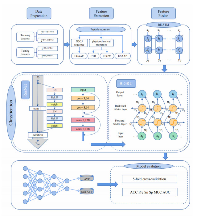
Human history is also the history of the fight against viral diseases. From the eradication of viruses to coexistence, advances in biomedicine have led to a more objective understanding of viruses and a corresponding increase in the tools and methods to combat them. More recently, antiviral peptides (AVPs) have been discovered, which due to their superior advantages, have achieved great impact as antiviral drugs. Therefore, it is very necessary to develop a prediction model to accurately identify AVPs. In this paper, we develop the iAVPs-ResBi model using k-spaced amino acid pairs (KSAAP), encoding based on grouped weight (EBGW), enhanced grouped amino acid composition (EGAAC) based on the N5C5 sequence, composition, transition and distribution (CTD) based on physicochemical properties for multi-feature extraction. Then we adopt bidirectional long short-term memory (BiLSTM) to fuse features for obtaining the most differentiated information from multiple original feature sets. Finally, the deep model is built by combining improved residual network and bidirectional gated recurrent unit (BiGRU) to perform classification. The results obtained are better than those of the existing methods, and the accuracies are 95.07, 98.07, 94.29 and 97.50% on the four datasets, which show that iAVPs-ResBi can be used as an effective tool for the identification of antiviral peptides. The datasets and codes are freely available at https://github.com/yunyunliang88/iAVPs-ResBi.

| [1] |
E. Domingo, Mechanisms of viral emergence, Vet. Res., 41 (2010), 38. https://doi.org/10.1051/vetres/2010010 doi: 10.1051/vetres/2010010

|
| [2] |
S. T. Nichol, J. Arikawa, Y. Kawaoka, Emerging viral diseases, Proc. Natl. Acad. Sci., 97 (2000), 12411–12412. https://doi.org/10.1073/pnas.210382297 doi: 10.1073/pnas.210382297
|
| [3] |
Q. Abid, T. Nishant, T. Himani, K. Manoj, AVPdb: a database of experimentally validated antiviral peptides targeting medically important viruses, Nucleic Acids Res., 42 (2014), D1147–D1153. https://doi.org/10.1093/nar/gkt1191 doi: 10.1093/nar/gkt1191
|
| [4] |
T. Phan. Genetic diversity and evolution of SARS-CoV2, Infect. Genet. Evol., 81 (2020), 104260. https://doi.org/10.1016/j.meegid.2020.104260 doi: 10.1016/j.meegid.2020.104260
|
| [5] |
E. Sherif, A. Maha, The potential of antimicrobial peptides as an antiviral therapy against COVID-19, ACS Pharmacol. Transl. Sci., 3 (2020), 780–782. https://doi.org/10.1021/acsptsci.0c00059 doi: 10.1021/acsptsci.0c00059
|
| [6] |
T. Uhlig, T. Kyprianou, F. G. Martinelli, C. A. Oppici, D. Heiligers, D. Hills, et al., The emergence of peptides in the pharmaceutical business: From exploration to exploitation, EuPA Open Proteomics, 4 (2014), 58–69. https://doi.org/10.1016/j.euprot.2014.05.003 doi: 10.1016/j.euprot.2014.05.003
|
| [7] |
L. Otvos, Peptide-based drug design: here and now, Methods Mol. Biol., 494 (2008), 1–8. https://doi.org/10.1007/978-1-59745-419-3 doi: 10.1007/978-1-59745-419-3
|
| [8] |
R. E. W. Hancock, H. G. Sahl, Antimicrobial and host-defense peptides as new anti-infective therapeutic strategies, Nat. Biotechnol., 24 (2006), 1551–1557. https://doi.org/10.1038/nbt1267 doi: 10.1038/nbt1267
|
| [9] |
A, Furka, F. Sebestyén, M. Asgedom, G. Dibó, General method for rapid synthesis of multicomponent peptide mixtures, Int. J. Pept. Protein Res., 37 (1991), 487–493. https://doi.org/10.1111/j.1399-3011.1991.tb00765.x doi: 10.1111/j.1399-3011.1991.tb00765.x
|
| [10] |
K. Bozovičar, T. Bratkovič, Evolving a peptide: library platforms and diversification strategies, Int. J. Mol. Sci., 21 (2019), 215. https://doi.org/10.3390/ijms21010215 doi: 10.3390/ijms21010215
|
| [11] |
Z. Y. Lou, Y. N. Sun, Z. H. Rao, Current progress in antiviral strategies. Trends Pharmacol. Sci., 35 (2014), 86–102. https://doi.org/10.1016/j.tips.2013.11.006 doi: 10.1016/j.tips.2013.11.006
|
| [12] |
F. Yu, L. Lu, L. Y. Du, X. J. Zhu, A. K. Debnath, S. Jiang, Approaches for identification of HIV-1 entry inhibitors targeting gp41 pocket, Viruses, 5 (2013), 127–149. https://doi.org/10.3390/v5010127 doi: 10.3390/v5010127
|
| [13] | C. K. McDonald, D. R. Kuritzkes, Human immunodeficiency virus type 1 protease inhibitors, Arch. Intern. Med., 157 (1997), 951–959. |
| [14] |
J. J. Kiser, C. Flexner, Direct-acting antiviral agents for hepatitis C virus infection, Annu. Rev. Pharmacol. Toxicol., 53 (2013), 427–449. https://doi.org/10.1146/annurev-pharmtox-011112-140254 doi: 10.1146/annurev-pharmtox-011112-140254
|
| [15] |
R. Eléonore, R. Jean-Christophe, B. Véronique, J. Corinne, P. Pierre, T, Noël, et al., Antiviral drug discovery strategy using combinatorial libraries of structurally constrained peptides, J. Virol., 78 (2004), 7410–7417. https://doi.org/10.1128/JVI.78.14.7410-7417.2004 doi: 10.1128/JVI.78.14.7410-7417.2004
|
| [16] |
G. Castel, M. Chtéoui, B. Heyd, N. Tordo, Phage display of combinatorial peptide libraries: application to antiviral research, Molecules, 16 (2011), 3499–3518. https://doi.org/10.3390/molecules16053499 doi: 10.3390/molecules16053499
|
| [17] |
M. F. Chew, K. S. Poh, C. L. Poh, Peptides as therapeutic agents for dengue virus, Int. J. Med. Sci., 14 (2017), 1342–1359. https://doi.org/10.7150/ijms.21875. doi: 10.7150/ijms.21875
|
| [18] | S. Saheli, Vaccination: the present and the future, Yale J. Biol. Med., 84 (2011), 353–359. |
| [19] |
H. B. Jiang, Y. D. Xu, L. Li, L. Y. Weng, Q. Wang, S. J. Zhang, et al., Inhibition of influenza virus replication by constrained peptides targeting nucleoprotein, Antiviral Chem. Chemother., 22 (2011), 119–130. https://doi.org/10.3851/IMP1902 doi: 10.3851/IMP1902
|
| [20] |
T. Nishant, Q. Abid, K. Manoj, AVPpred: collection and prediction of highly effective antiviral peptides, Nucleic Acids Res., 40 (2012), W199–W204. https://doi.org/10.1093/nar/gks450 doi: 10.1093/nar/gks450
|
| [21] |
K. Y. Chang, J. R. Yang, Analysis and prediction of highly effective antiviral peptides based on random forests, PloS One, 8 (2013), e70166. https://doi.org/10.1371/journal.pone.0070166 doi: 10.1371/journal.pone.0070166
|
| [22] |
M. Zare, H. Mohabatkar, F. K. Faramarzi, M. M. Beigi, M. Behbahani, Using Chou's pseudo amino acid composition and machine learning method to predict the antiviral peptides, Open Bioinf. J., 9 (2015), 13–19. https://doi.org/10.2174/1875036201509010013 doi: 10.2174/1875036201509010013
|
| [23] |
B. F. J. Lissabet, H. L. Belén, G. J. Farias, AntiVPP 1.0: A portable tool for prediction of antiviral peptides, Comput. Biol. Med., 107 (2019), 127–130. https://doi.org/10.1016/j.compbiomed.2019.02.011 doi: 10.1016/j.compbiomed.2019.02.011
|
| [24] |
N. Schaduangrat, C. Nantasenamat, V. Prachayasittikul, W. Shoombuatong, Meta-iAVP: a sequence-based meta-predictor for improving the prediction of antiviral peptides using effective feature representation, Int. J. Mol. Sci., 20 (2019), 5743. https://doi.org/10.3390/ijms20225743 doi: 10.3390/ijms20225743
|
| [25] |
S. C. Abu, M. R. Sarah, K. H. Kylene, B. Barney, M. W. R. Bobbie-Jo, Better understanding and prediction of antiviral peptides through primary and secondary structure feature importance, Sci. Rep., 10 (2020), 19260. https://doi.org/10.1038/s41598-020-76161-8 doi: 10.1038/s41598-020-76161-8
|
| [26] |
J. W. Li, Y. Q. Pu, J. J. Tang, Q. Zou, F. Guo, DeepAVP: a dual-channel deep neural network for identifying variable-length antiviral peptides, IEEE J. Biomed. Health, 24 (2020), 3012–3019. https://doi.org/10.1109/JBHI.2020.2977091 doi: 10.1109/JBHI.2020.2977091
|
| [27] |
Y. X. Pang, Z. Wang, J. H. Jhong, T. Y. Lee, Identifying anti-coronavirus peptides by incorporating different negative datasets and imbalanced learning strategies, Briefings Bioinf., 22 (2021), 1085–1095. https://doi.org/10.1093/bib/bbaa423 doi: 10.1093/bib/bbaa423
|
| [28] |
Y. Pang, L. Yao, J. H. Jhong, Z. Wang, T. Y. Lee, AVPIden: a new scheme for identification and functional prediction of antiviral peptides based on machine learning approaches, Brief. Bioinform., 22 (2021), bbab263. https://doi.org/10.1093/bib/bbab263 doi: 10.1093/bib/bbab263
|
| [29] |
P. B. Timmons, C. M. Hewage, ENNAVIA is a novel method which employs neural networks for antiviral and anti-coronavirus activity prediction for therapeutic peptides, Briefings Bioinf., 22 (2021), bbab258. https://doi.org/10.1093/bib/bbab258 doi: 10.1093/bib/bbab258
|
| [30] |
G. Agarwal, R. Gabrani, Antiviral peptides: identification and validation, Int. J. Pept. Res. Ther., 27 (2021), 149–168. https://doi.org/10.1007/s10989-020-10072-0 doi: 10.1007/s10989-020-10072-0
|
| [31] |
P. Charoenkwan, N. Anuwongcharoen, C. Nantasenamat, M. M. Hasan, W. Shoombuatong, In silico approaches for the prediction and analysis of antiviral peptides: a review, Curr. Pharm. Design, 27 (2021), 2180–2188. https://doi.org/10.2174/1381612826666201102105827 doi: 10.2174/1381612826666201102105827
|
| [32] |
B. Manavalan, S. Basith, G. Lee, Comparative analysis of machine learning-based approaches for identifying therapeutic peptides targeting SARS-CoV-2, Briefings Bioinf., 23 (2022), bbab412. https://doi.org/10.1093/bib/bbab412 doi: 10.1093/bib/bbab412
|
| [33] |
H. Kurata, S. Tsukiyama, B. Manavalan, iACVP: markedly enhanced identification of anti-coronavirus peptides using a dataset-specific word2vec model, Briefings Bioinf., 23 (2022), bbac265. https://doi.org/10.1093/bib/bbac265 doi: 10.1093/bib/bbac265
|
| [34] |
M. K. Pirtskhalava, A. A. Amstrong, M. Grigolava, M. Chubinidze, E. Alimbarashvili, B. M. Vishnepolsky, DBAASP v3: database of antimicrobial/cytotoxic activity and structure of peptides as a resource for development of new therapeutics, Nucleic. Acids Res., 49 (2021), D288–D297. https://doi.org/10.1093/nar/gkaa991 doi: 10.1093/nar/gkaa991
|
| [35] |
F. H. Waghu, L. Gopi, R. S. Barai, P. Ramteke, B. Nizami, S. Idicula-Thomas, CAMP: Collection of sequences and structures of antimicrobial peptides, Nucleic. Acids Res., 42 (2014), D1154–D1158. https://doi.org/10.1093/nar/gkt1157 doi: 10.1093/nar/gkt1157
|
| [36] |
G. S. Wang, X. Li, Z. Wang, APD3: the antimicrobial peptide database as a tool for research and education, Nucleic. Acids Res., 44 (2016), D1087–D1093. https://doi.org/10.1093/nar/gkv1278 doi: 10.1093/nar/gkv1278
|
| [37] |
S. Lata, N. K. Mishra, G. P. S. Raghava, AntiBP2: improved version of antibacterial peptide prediction, BMC Bioinf., 11 (2010), S19. https://doi.org/10.1186/1471-2105-11-S1-S19 doi: 10.1186/1471-2105-11-S1-S19
|
| [38] |
N. Bupi, V. K. Sangaraju, L. T. Phan, A. Lal, T. T. B. Vo, P. T. Ho, et al., An effective integrated machine learning framework for identifying severity of tomato yellow leaf curl virus and their experimental validation, Research, 6 (2023), 16. https://doi.org/10.34133/research.0016 doi: 10.34133/research.0016
|
| [39] |
H. Y. Shi, S. L. Zhang, Accurate prediction of anti-hypertensive peptides based on convolutional neural network and gated recurrent unit, Interdiscip. Sci., 14 (2022), 879–894. https://doi.org/10.1007/s12539-022-00521-3 doi: 10.1007/s12539-022-00521-3
|
| [40] |
S. L. Zhang, X. J. Li, Pep-CNN: An improved convolutional neural network for predicting therapeutic peptides, Chemometr. Intell. Lab., 221 (2022), 104490. https://doi.org/10.1016/j.chemolab.2022.104490 doi: 10.1016/j.chemolab.2022.104490
|
| [41] |
M. M. Hasan, Y. Zhou, X. T. Lu, J. Y. Li, J. N. Song, Z. D. Zhang, Computational identification of protein pupylation sites by using profile-based composition of k-spaced amino acid pairs, PloS One, 10 (2015), e0129635. https://doi.org/10.1371/journal.pone.0129635 doi: 10.1371/journal.pone.0129635
|
| [42] |
Z. Ju, J. Z. Cao, Prediction of protein N-formylation using the composition of k-spaced amino acid pairs, Anal. Biochem., 534 (2017), 40–45. https://doi.org/10.1016/j.ab.2017.07.011 doi: 10.1016/j.ab.2017.07.011
|
| [43] |
Z. Ju, S. Y. Wang, Prediction of lysine formylation sites using the composition of k-spaced amino acid pairs via Chou's 5-steps rule and general pseudo components, Genomics, 112 (2020), 859–866. https://doi.org/10.1016/j.ygeno.2019.05.027 doi: 10.1016/j.ygeno.2019.05.027
|
| [44] |
M. M. Hasan, M. S. Khatun, M. N. H. Mollah, Y. Cao, D. J. Guo, NTyroSite: Computational identification of protein nitrotyrosine sites using sequence evolutionary features, Molecules, 23 (2018), 1667. https://doi.org/10.3390/molecules23071667 doi: 10.3390/molecules23071667
|
| [45] |
H. L. Fu, Y. X. Yang, X. B. Wang, H. Wang, Y. Xu, DeepUbi: a deep learning framework for prediction of ubiquitination sites in proteins, BMC Bioinf., 20 (2019), 86. https://doi.org/10.1186/s12859-019-2677-9 doi: 10.1186/s12859-019-2677-9
|
| [46] |
J. N. Song, Y. N. Wang, F. Y. Li, T. Akutsu, N. D. Rawlings, G. I. Webb, K. C. Chou, iProt-Sub: a comprehensive package for accurately mapping and predicting protease-specific substrates and cleavage sites, Briefings Bioinf., 20 (2019), 638–658. https://doi.org/10.1093/bib/bby028 doi: 10.1093/bib/bby028
|
| [47] |
M. Usman, S. Khan, J. A. Lee, Afp-lse: Antifreeze proteins prediction using latent space encoding of composition of k-spaced amino acid pairs, Sci. Rep., 10 (2020), 7197. https://doi.org/10.1038/s41598-020-63259-2 doi: 10.1038/s41598-020-63259-2
|
| [48] |
Z. Chen, P. Zhao, F. Y. Li, A. Leier, T. T. Marquez-Lago, Y. N. Wang, et al., iFeature: a python package and web server for features extraction and selection from protein and peptide sequences, Bioinformatics, 34 (2018), 2499–2502. https://doi.org/10.1093/bioinformatics/bty140 doi: 10.1093/bioinformatics/bty140
|
| [49] |
Y. Zhu, C. Z. Jia, F. Y. Li, J. N. Song, Inspector: a lysine succinylation predictor based on edited nearest-neighbor undersampling and adaptive synthetic oversampling, Anal. Biochem., 593 (2020), 113592. https://doi.org/10.1016/j.ab.2020.113592 doi: 10.1016/j.ab.2020.113592
|
| [50] |
C. R. Chung, T. R. Kuo, L. C. Wu, T. Y. Lee, J. T. Horng, Characterization and identification of antimicrobial peptides with different functional activities, Briefings Bioinf., 21 (2020), 1098–1114. https://doi.org/10.1093/bib/bbz043 doi: 10.1093/bib/bbz043
|
| [51] |
Y. J. Wang, Q. Zhang, M. A. Sun, D. J. Guo, High-accuracy prediction of bacterial type Ⅲ secreted effectors based on position specific amino acid composition profiles, Bioinformatics, 27 (2011), 777–784. https://doi.org/10.1093/bioinformatics/btr021 doi: 10.1093/bioinformatics/btr021
|
| [52] |
T. Y. Lee, Z. Q. Lin, S. J. Hsieh, N. A. Bretana, C. T. Lu, Exploiting maximal dependence decomposition to identify conserved motifs from a group of aligned signal sequences, Bioinformatics, 27 (2011), 1780–1787. https://doi.org/10.1093/bioinformatics/btr291 doi: 10.1093/bioinformatics/btr291
|
| [53] |
X. Y. Wang, B. Yu, A. J. Ma, C. Chen, B. Q. Liu, Q. Ma, Protein-protein interaction sites prediction by ensemble random forests with synthetic minority oversampling technique, Bioinformatics, 35 (2019), 2395–2402. https://doi.org/10.1093/bioinformatics/bty995 doi: 10.1093/bioinformatics/bty995
|
| [54] |
B. G. Tian, X. Wu, C. Chen, W. Y. Qiu, Q. Ma, B. Yu, Predicting protein-protein interactions by fusing various Chou's pseudo components and using wavelet denoising approach, J. Theor. Biol., 462 (2019), 329–346. https://doi.org/10.1016/j.jtbi.2018.11.011 doi: 10.1016/j.jtbi.2018.11.011
|
| [55] |
Z. H. Zhang, Z. H. Wang, Z. R. Zhang, Y. X. Wang, A novel method for apoptosis protein subcellular localization prediction combining encoding based on grouped weight and support vector machine, FEBS Lett., 580 (2006), 6169–6174. https://doi.org/10.1016/j.febslet.2006.10.017 doi: 10.1016/j.febslet.2006.10.017
|
| [56] |
I. Dubchak, I. Muchnik, S. R. Holbrook, S. H. Kim, Prediction of protein folding class using global description of amino acid sequence, Proc. Natl. Acad. Sci., 92 (1995), 8700–8704. https://doi.org/10.2307/2368330 doi: 10.2307/2368330
|
| [57] |
Z. R. Li, H. H. Lin, L. Y. Han, L. Jiang, X. Chen, Y. Z. Chen, PROFEAT: a web server for computing structural and physicochemical features of proteins and peptides from amino acid sequence, Nucleic. Acids Res., 34 (2006), W32–W37. https://doi.org/10.1093/nar/gkl305 doi: 10.1093/nar/gkl305
|
| [58] |
H. Lv, F. Y. Dao, Z. X. Guan, H. Yang, Y. W. Li, H. Lin, Deep-Kcr: accurate detection of lysine crotonylation sites using deep learning method, Briefings Bioinf., 22 (2021), bbaa255. https://doi.org/10.1093/bib/bbaa255 doi: 10.1093/bib/bbaa255
|
| [59] |
S. Hochreiter, J. Schmidhuber, Long short-term memory, Neural Comput., 9 (1997), 1735–1780. https://doi.org/10.1162/neco.1997.9.8.1735 doi: 10.1162/neco.1997.9.8.1735
|
| [60] |
A. Graves, J. Schmidhuber, Framewise phoneme classification with bidirectional LSTM and other neural network architectures, Neural Networks, 18 (2005), 602–610. https://doi.org/10.1016/j.neunet.2005.06.042 doi: 10.1016/j.neunet.2005.06.042
|
| [61] |
J. W. Li, Y. Q. Pu, J. J. Tang, Q. Zou, F. Guo, DeepATT: a hybrid category attention neural network for identifying functional effects of DNA sequences, Briefings Bioinf., 22 (2021), bbaa159. https://doi.org/10.1093/bib/bbaa159 doi: 10.1093/bib/bbaa159
|
| [62] |
K. M. He, X. Y. Zhang, S. Q. Ren, J. Sun, Deep residual learning for image recognition, Comput. Sci., (2016), 770–778. https://doi.org/10.48550/arXiv.1512.03385 doi: 10.48550/arXiv.1512.03385
|
| [63] | R. Zhou, X. Q. Hu, B. Yuan, Q. W. Xu, Lithology classification system for well logging based on bidirectional gated recurrent unit, in 2021 4th International conference on artificial intelligence and big data (ICAIBD), (2021), 599–603. https://doi.org/10.1109/ICAIBD51990.2021.9459000 |
| [64] |
S. L. Zhang, Y. Y. Jing, PreVFs-RG: A deep hybrid model for identifying virulence factors based on residual block and gated recurrent unit, IEEE/ACM Trans. Comput. Biol. Bioinf., 20 (2022), 1926–1934. https://doi.org/10.1109/TCBB.2022.3223038 doi: 10.1109/TCBB.2022.3223038
|
| [65] | K. M. He, X. Y. Zhang, S. Q. Ren, J. Sun, Identity mappings in deep residual networks, in Computer Vision–ECCV 2016: 14th European Conference, (2016), 630–645. https://doi.org/10.48550/arXiv.1603.05027 |
| [66] | K. Cho, B. V. Merrienboer, C. Gulcehre, D. Bahdanau, F. Bougares, H. Schwenk, et al., Learning phrase representations using RNN encoder-decoder for statistical machine translation, preprint, arXiv: 1406.1078. https://doi.org/10.48550/arXiv.1406.1078 |
| [67] |
K. Abdelli, J. Y. Cho, F. Azendorf, H. Griesser, C. Tropschug, S. Pachnicke, Machine-learning-based anomaly detection in optical fiber monitoring, J. Opt. Commun. Networking, 14 (2022), 365–375. https://doi.org/10.1364/JOCN.451289 doi: 10.1364/JOCN.451289
|
| [68] |
Q. H. Kha, Q. T. Ho, N. Q. K. Le, Identifying SNARE proteins using an alignment-free method based on multiscan convolutional neural network and PSSM profiles, J. Chem. Inf. Model., 62 (2022), 4820–4826. https://doi.org/10.1021/acs.jcim.2c01034 doi: 10.1021/acs.jcim.2c01034
|
| [69] |
N. Q. K. Le, T. T. D. Nguyen, Y. Y. Ou, Identifying the molecular functions of electron transport proteins using radial basis function networks and biochemical properties, J. Mol. Graph. Model., 73 (2017), 166–178. https://doi.org/10.1016/j.jmgm.2017.01.003 doi: 10.1016/j.jmgm.2017.01.003
|
| [70] |
W. Shoombuatong, S. Basith, T. Pitti, G. Lee, B. Manavalan, THRONE: a new approach for accurate prediction of human RNA N7-methylguanosine sites, J. Mol. Biol., 434 (2022), 167549. https://doi.org/10.1016/j.jmb.2022.167549 doi: 10.1016/j.jmb.2022.167549
|
| [71] |
L. Y. Wei, W. J. He, A. Malik, R. Su, L. Z. Cui, B. Manavalan, Computational prediction and interpretation of cell-specific replication origin sites from multiple eukaryotes by exploiting stacking framework, Briefings Bioinf., 22 (2021), bbaa275. https://doi.org/10.1093/bib/bbaa275 doi: 10.1093/bib/bbaa275
|
| [72] |
M. M. Hasan, S. Tsukiyama, J. Y. Cho, H. Kurata, M. A. Alam, X. W. Liu, et al., Deepm5C: a deep-learning-based hybrid framework for identifying human RNA N5-methylcytosine sites using a stacking strategy, Mol. Ther., 30 (2022), 2856–2867. https://doi.org/10.1016/j.ymthe.2022.05.001 doi: 10.1016/j.ymthe.2022.05.001
|
| [73] |
P. Charoenkwan, W. Chiangjong, C. Nantasenamat, M. M. Hasan, B. Manavalan, W. Shoombuatong, StackIL6: a stacking ensemble model for improving the prediction of IL-6 inducing peptides, Briefings Bioinf., 22 (2021), bbab172. https://doi.org/10.1093/bib/bbab172 doi: 10.1093/bib/bbab172
|
| [74] |
V. Vacic, L. M. Iakoucheva, P. Radivojac, Two Sample Logo: a graphical representation of the differences between two sets of sequence alignments, Bioinformatics, 22 (2006), 1536–1537. https://doi.org/10.1093/bioinformatics/btl151 doi: 10.1093/bioinformatics/btl151
|
| [75] |
M. Y. Liu, H. M. Liu, T. Wu, Y. X. Zhu, Y. W. Zhou, Z. R. Huang, et al., ACP‑Dnnel: anti‑coronavirus peptides' prediction based on deep neural network ensemble learning, Amino Acids, 55 (2023), 1121–1136. https://doi.org/10.1007/s00726-023-03300-6 doi: 10.1007/s00726-023-03300-6
|


Figures(5) / Tables(7)

Xinyan Ma, Yunyun Liang, Shengli Zhang. iAVPs-ResBi: Identifying antiviral peptides by using deep residual network and bidirectional gated recurrent unit[J]. Mathematical Biosciences and Engineering, 2023, 20(12): 21563-21587. doi: 10.3934/mbe.2023954


 DownLoad: