Analysis of a mathematical model for the spreading of the monkeypox virus with constant proportional-Caputo derivative operator

Jutarat Kongson; Chatthai Thaiprayoon; Weerawat Sudsutad; Jutarat Kongson; Chatthai Thaiprayoon; Weerawat Sudsutad

doi:10.3934/math.2025187

AIMS Mathematics

2025, Volume 10, Issue 2: 4000-4039. doi: 10.3934/math.2025187

Previous Article Next Article

Research article

Analysis of a mathematical model for the spreading of the monkeypox virus with constant proportional-Caputo derivative operator

1.
Research Group of Theoretical and Computational Applied Science, Department of Mathematics, Faculty of Science, Burapha University, Chonburi 20131, Thailand
2.
Department of Statistics, Faculty of Science, Ramkhamhaeng University, Bangkok 10240, Thailand

Received: 22 November 2024 Revised: 08 February 2025 Accepted: 18 February 2025 Published: 27 February 2025
MSC : 26A33, 34A08, 65L09, 92D25, 92D30

This work comprehensively analyzed the monkeypox virus utilizing a deterministic mathematical model within a constant proportional-Caputo derivative framework. The suggested model considered the interplay of human and rodent populations by incorporating certain realistic vaccination parameters. Our study was a testament to the thoroughness of this work. We explored the uniqueness result using Banach's contraction principle. The solution's positivity and boundedness were studied in detail, as were the basic reproduction number and the stability analysis of the system's equilibrium conditions. We performed a variety of Ulam's stability analyses to guarantee the solution existed. Additionally, we implemented a decomposition formula to obtain the numerical scheme. This numerical approach allowed for numerical simulation as a graphical representation for certain real data sets and different parameter values in order to understand the model's dynamic behavior.
- monkeypox disease,
- constant proportional-Caputo,
- Ulam stability,
- numerical algorithm,
- basic reproduction number
Citation: Jutarat Kongson, Chatthai Thaiprayoon, Weerawat Sudsutad. Analysis of a mathematical model for the spreading of the monkeypox virus with constant proportional-Caputo derivative operator[J]. AIMS Mathematics, 2025, 10(2): 4000-4039. doi: 10.3934/math.2025187

Related Papers:

Abstract

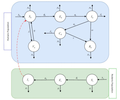
This work comprehensively analyzed the monkeypox virus utilizing a deterministic mathematical model within a constant proportional-Caputo derivative framework. The suggested model considered the interplay of human and rodent populations by incorporating certain realistic vaccination parameters. Our study was a testament to the thoroughness of this work. We explored the uniqueness result using Banach's contraction principle. The solution's positivity and boundedness were studied in detail, as were the basic reproduction number and the stability analysis of the system's equilibrium conditions. We performed a variety of Ulam's stability analyses to guarantee the solution existed. Additionally, we implemented a decomposition formula to obtain the numerical scheme. This numerical approach allowed for numerical simulation as a graphical representation for certain real data sets and different parameter values in order to understand the model's dynamic behavior.

References

[1]	World Health Organization, Monkeypox outbreak 2022, World Health Organization, 2022. Available from: https://www.who.int/emergencies/situations/monkeypox-oubreak-2022.
[2]	S. Jayswal, J. Kakadiya, A narrative review of pox: smallpox vs monkeypox, The Egyptian Journal of Internal Medicine, 34 (2022), 90. http://doi.org/10.1186/s43162-022-00174-0 doi: 10.1186/s43162-022-00174-0
[3]	Z. Jezek, F. Fenner, Human monkeypox, New York: Karger, 1988.
[4]	S. Essbauer, M. Pfeffer, H. Meyer, Zoonotic poxviruses, Vet. Microbiol., 140 (2010), 229–236. https://doi.org/10.1016/j.vetmic.2009.08.026
[5]	A. W. Rimoin, P. M. Mulembakani, S. C. Johnston, J. O. L. Smith, N. K. Kisalu, T. L. Kinkela, et al., Major increase in human monkeypox incidence 30 years after smallpox vaccination campaigns cease in the Democratic Republic of Congo, Proc. Natl. Acad. Sci., 107 (2010), 16262–16267. https://doi.org/10.1073/pnas.1005769107 doi: 10.1073/pnas.1005769107
[6]	S. Usman, I. I. Adamu, Modeling the transmission dynamics of the monkeypox virus infection with treatment and vaccination interventions, Journal of Applied Mathematics and Physics, 5 (2017), 2335–2353. https://doi.org/10.4236/jamp.2017.512191 doi: 10.4236/jamp.2017.512191
[7]	A. Elsonbaty, W. Adel, A. Aldurayhim, A. El-Mesady, Mathematical modeling and analysis of a novel monkeypox virus spread integrating imperfect vaccination and nonlinear incidence rates, Ain Shams Eng. J., 15 (2024), 102451. https://doi.org/10.1016/j.asej.2023.102451 doi: 10.1016/j.asej.2023.102451
[8]	S. A. Somma, N. I. Akinwande, U. D. Chado, A mathematical model of monkeypox virus transmission dynamics, Ife Journal of Science, 21 (2019), 195–204. https://doi.org/10.4314/ijs.v21i1.17 doi: 10.4314/ijs.v21i1.17
[9]	O. J. Peter, S. Kumar, N. Kumari, F. A. Oguntolu, K. Oshinubi, R. Musa, Transmission dynamics of monkeypox virus: a mathematical modelling approach, Model. Earth Syst. Environ., 8 (2022), 3423–3434. https://doi.org/10.1007/s40808-021-01313-2 doi: 10.1007/s40808-021-01313-2
[10]	O. J. Peter, C. E. Madubueze, M. M. Ojo, F. A. Oguntolu, T. A. Ayoola, Modeling and optimal control of monkeypox with cost-effective strategies, Model. Earth Syst. Environ., 9 (2023), 1989–2007. https://doi.org/10.1007/s40808-022-01607-z doi: 10.1007/s40808-022-01607-z
[11]	O. J. Peter, A. Abidemi, M. M. Ojo, T. A. Ayoola, Mathematical model and analysis of monkeypox with control strategies, Eur. Phys. J. Plus, 138 (2023), 242. https://doi.org/10.1140/epjp/s13360-023-03865-x doi: 10.1140/epjp/s13360-023-03865-x
[12]	C. P. Bhunu, S. Mushayabasa, Modelling the transmission dynamics of pox-like infections, IAENG International Journal of Applied Mathematics, 41 (2011), 141–149.
[13]	L. E. Depero, E. Bontempi, Comparing the spreading characteristics of monkeypox (MPX) and COVID-19: insights from a quantitative model, Environ. Res., 235 (2023), 116521. https://doi.org/10.1016/j.envres.2023.116521 doi: 10.1016/j.envres.2023.116521
[14]	N. Z. Alshahrani, F. Alzahrani, A. M. Alarifi, M. R. Algethami, M. N. Alhumam, H. A. M. Ayied, et al., Assessment of knowledge of monkeypox viral infection among the general population in Saudi Arabia, Pathogens, 11 (2022), 904. https://doi.org/10.3390/pathogens11080904 doi: 10.3390/pathogens11080904
[15]	D. Baleanu, A. Fernandez, On fractional operators and their classifications, Mathematics, 7 (2019), 830. https://doi.org/10.3390/math7090830 doi: 10.3390/math7090830
[16]	K. Diethelm, The analysis of fractional differential equations: an application-oriented exposition using differential operators of Caputo type, Berlin: Springer, 2010. https://doi.org/10.1007/978-3-642-14574-2
[17]	U. N. Katugampola, New approach to a generalized fractional integral, Appl. Math. Comput., 218 (2011), 860–865. https://doi.org/10.1016/j.amc.2011.03.062 doi: 10.1016/j.amc.2011.03.062
[18]	A. Atangana, D. Baleanu, New fractional derivatives with nonlocal and non-singular kernel, theory, and application to heat transfer model, Therm. Sci., 20 (2016), 763–769. https://doi.org/10.2298/TSCI160111018A doi: 10.2298/TSCI160111018A
[19]	A. Atangana, Fractal-fractional differentiation and integration: connecting fractal calculus and fractional calculus to predict complex system, Chaos Soliton. Fract., 102 (2017), 396–406. https://doi.org/10.1016/j.chaos.2017.04.027 doi: 10.1016/j.chaos.2017.04.027
[20]	R. Kamocki, A new representation formula for the Hilfer fractional derivative and its application, J. Comput. Appl. Math., 308 (2016), 39–45. https://doi.org/10.1016/j.cam.2016.05.014 doi: 10.1016/j.cam.2016.05.014
[21]	D. Baleanu, A. Fernandez, A. Akgül, On a fractional operator combining proportional and classical differintegrals, Mathematics, 8 (2020), 360. https://doi.org/10.3390/math8030360 doi: 10.3390/math8030360
[22]	W. Sudsutad, J. Kongson, C. Thaiprayoon, On generalized $(k, \psi)$-Hilfer proportional fractional operator and its applications to the higher-order Cauchy problem, Bound. Value Probl., 2024 (2024), 83. https://doi.org/10.1186/s13661-024-01891-x doi: 10.1186/s13661-024-01891-x
[23]	N. H. Sweilam, S. M. Al-Mekhlafi, D. Baleanu, A hybrid fractional optimal control for a novel Coronavirus (2019-nCov) mathematical model, J. Adv. Res., 32 (2021), 149–160. https://doi.org/10.1016/j.jare.2020.08.006 doi: 10.1016/j.jare.2020.08.006
[24]	H. Gnerhan, H. Dutta, M. A. Dokuyucu, W. Adel, Analysis of a fractional HIV model with Caputo and constant proportional Caputo operators, Chaos Soliton. Fract., 139 (2020), 110053. https://doi.org/10.1016/j.chaos.2020.110053 doi: 10.1016/j.chaos.2020.110053
[25]	M. Farman, A. Shehzad, A. Akgül, D. Baleanu, M. D. la Sen, Modelling and analysis of a measles epidemic model with the constant proportional Caputo operator, Symmetry, 15 (2023), 468. https://doi.org/10.3390/sym15020468 doi: 10.3390/sym15020468
[26]	M. Farman, C. Alfiniyah, A constant proportional caputo operator for modeling childhood disease epidemics, Decision Analytics Journal, 10 (2024), 100393. https://doi.org/10.1016/j.dajour.2023.100393 doi: 10.1016/j.dajour.2023.100393
[27]	M. Arif, P. Kumam, W. Watthayu, Analysis of constant proportional Caputo operator on the unsteady Oldroyd-B fluid flow with Newtonian heating and non-uniform temperature, Z. Angew. Math. Mech., 104 (2024), e202300048. https://doi.org/10.1002/zamm.202300048 doi: 10.1002/zamm.202300048
[28]	A. El-Mesady, O. J. Peter, A. Omame, F. A. Oguntolu, Mathematical analysis of a novel fractional order vaccination model for Tuberculosis incorporating susceptible class with underlying ailment, Int. J. Model. Simul., in press. https://doi.org/10.1080/02286203.2024.2371684
[29]	O. J. Peter, N. D. Fahrani, Fatmawati, Windarto, C. W. Chukwu, A fractional derivative modeling study for measles infection with double dose vaccination, Healthcare Analytics, 4 (2023), 100231. https://doi.org/10.1016/j.health.2023.100231 doi: 10.1016/j.health.2023.100231
[30]	O. J. Peter, A. Yusuf, M. M. Ojo, S. Kumar, N. Kumari, F. A. Oguntolu, A mathematical model analysis of meningitis with treatment and vaccination in fractional derivatives, Int. J. Appl. Comput. Math., 8 (2022), 117. https://doi.org/10.1007/s40819-022-01317-1 doi: 10.1007/s40819-022-01317-1
[31]	O. J. Peter, A. Yusuf, K. Oshinubi, F. A. Oguntolu, J. O. Lawal, A. I. Abioye, et al., Fractional order of pneumococcal pneumonia infection model with Caputo Fabrizio operator, Results Phys., 29 (2021), 104581. https://doi.org/10.1016/j.rinp.2021.104581 doi: 10.1016/j.rinp.2021.104581
[32]	O. J. Peter, Transmission dynamics of fractional order brucellosis model using Caputo-Fabrizio operator, Int. J. Differ. Equat., 2020 (2020), 2791380. https://doi.org/10.1155/2020/2791380 doi: 10.1155/2020/2791380
[33]	O. J. Peter, F. A. Oguntolu, M. M. Ojo, A. O. Oyeniyi, R. Jan, I. Khan, Fractional order mathematical model of monkeypox transmission dynamics, Phys. Scr., 97 (2022), 084005. https://doi.org/10.1088/1402-4896/ac7ebc doi: 10.1088/1402-4896/ac7ebc
[34]	M. Ngungu, E. Addai, A. Adeniji, U. M. Adam, K. Oshinubi, Mathematical epidemiological modeling and analysis of monkeypox dynamism with non-pharmaceutical intervention using real data from United Kingdom, Front. Public Health, 11 (2023), 1101436. https://doi.org/10.3389/fpubh.2023.1101436 doi: 10.3389/fpubh.2023.1101436
[35]	F. A. Wireko, I. K. Adu, C. Sebil, J. K. K. Asamoah, A fractal-fractional order model for exploring the dynamics of Monkeypox disease, Decision Analytics Journal, 8 (2023), 100300. https://doi.org/10.1016/j.dajour.2023.100300 doi: 10.1016/j.dajour.2023.100300
[36]	W. Sudsutad, C. Thaiprayoon, J. Kongson, W. Sae-Dan, A mathematical model for fractal-fractional monkeypox disease and its application to real data, AIMS Math., 9 (2024), 8516–8563. https://doi.org/10.3934/math.2024414 doi: 10.3934/math.2024414
[37]	A. El-Mesady, A. Elsonbaty, W. Adel, On nonlinear dynamics of a fractional order monkeypox virus model, Chaos Soliton. Fract., 164 (2022), 112716. https://doi.org/10.1016/j.chaos.2022.112716 doi: 10.1016/j.chaos.2022.112716
[38]	M. A. Qurashi, S. Rashid, A. M. Alshehri, F. Jarad, F. Safdar, New numerical dynamics of the fractional monkeypox virus model transmission pertaining to nonsingular kernels, Mathematical Biosciences and Engineering, 20 (2022), 402–436. https://doi.org/10.3934/mbe.2023019 doi: 10.3934/mbe.2023019
[39]	N. Zhang, E. Addai, L. Zhang, M. Ngungu, E. Marinda, J. K. K. Asamoah, Fractional modeling and numerical simulation for unfolding marburg-monkeypox virus co-infection transmission, Fractals, 31 (2023), 2350086. https://doi.org/10.1142/S0218348X2350086X doi: 10.1142/S0218348X2350086X
[40]	B. Liu, S. Farid, S. Ullah, M. Altanji, R. Nawaz, S. W. Teklu, Mathematical assessment of monkeypox disease with the impact of vaccination using a fractional epidemiological modeling approach, Sci. Rep., 13 (2023), 13550. https://doi.org/10.1038/s41598-023-40745-x doi: 10.1038/s41598-023-40745-x
[41]	A. S. Biswas, B. H. Aslam, P. K. Tiwari, Mathematical modeling of a novel fractional-order monkeypox model using the Atangana-Baleanu derivative, Phys. Fluids, 35 (2023), 117130. https://doi.org/10.1063/5.0174767 doi: 10.1063/5.0174767
[42]	S. Okyere, J. Ackora-Prah, Modeling and analysis of monkeypox disease using fractional derivatives, Results Eng., 17 (2023), 100786. https://doi.org/10.1016/j.rineng.2022.100786 doi: 10.1016/j.rineng.2022.100786
[43]	A. Atangana, S. I. Araz, New numerical scheme with Newton polynomial: theory, methods, and applications, 1 Eds., Elsevier, 2021. https://doi.org/10.1016/C2020-0-02711-8
[44]	V. S. Erturk, P. Kumar, Solution of a COVID-19 model via new generalized Caputo-type fractional derivatives, Chaos Soliton. Fract., 139 (2020), 110280. https://doi.org/10.1016/j.chaos.2020.110280 doi: 10.1016/j.chaos.2020.110280
[45]	H. Najafi, S. Etemad, N. Patanarapeelert, J. K. K. Asamoah, S. Rezapour, T. Sitthiwirattham, A study on dynamics of CD$4+$ T-cells under the effect of HIV-1 infection based on a mathematical fractal-fractional model via the Adams-Bashforth scheme and Newton polynomials, Mathematics, 10 (2022), 1366. https://doi.org/10.3390/math10091366 doi: 10.3390/math10091366
[46]	D. Boucenna, D. Baleanu, A. B. Makhloufd, A. M. Nagy, Analysis and numerical solution of the generalized proportional fractional Cauchy problem, Appl. Numer. Math., 167 (2021), 173–186. https://doi.org/10.1016/j.apnum.2021.04.015 doi: 10.1016/j.apnum.2021.04.015
[47]	W. Sudsutad, C. Thaiprayoon, A. Aphithana, J. Kongson, W. Sae-Dan, Qualitative results and numerical approximations of the $(k, \psi)$-Caputo proportional fractional differential equations and applications to blood alcohol levels model, AIMS Math., 9 (2024), 34013–34041. https://doi.org/10.3934/math.20241622 doi: 10.3934/math.20241622
[48]	S. M. Ulam, A collection of mathematical problems, New York: Interscience, 1960.
[49]	D. H. Hyers, On the stability of the linear functional equation, Proc. Natl. Acad. Sci., 27 (1941), 222–224. https://doi.org/10.1073/pnas.27.4.222 doi: 10.1073/pnas.27.4.222
[50]	T. M. Rassias, On the stability of linear mappings in Banach spaces, Proc. Amer. Math. Soc., 72 (1978), 297–300. https://doi.org/10.1090/S0002-9939-1978-0507327-1 doi: 10.1090/S0002-9939-1978-0507327-1
[51]	J. Wang, X. Li, $E_\alpha$-Ulam type stability of fractional order ordinary differential equations, J. Appl. Math. Comput., 45 (2014), 449–459. https://doi.org/10.1007/s12190-013-0731-8 doi: 10.1007/s12190-013-0731-8
[52]	I. Podlubny, Fractional differential equations, New York: Academic Press, 1999.
[53]	G. O. Fosu, E. Akweittey, A. S. Albert, Next-generation matrices and basic reproductive numbers for all phases of the coronavirus disease, Open J. Math. Sci., 4 (2020), 261–272. https://doi.org/10.2139/ssrn.3595958 doi: 10.2139/ssrn.3595958
[54]	A. Granas, J. Dugundji, Fixed point theory, New York: Springer, 2003. https://doi.org/10.1007/978-0-387-21593-8
[55]	Worldometer, United States population (accessed Nov 2022), Worldometer, 2022. Available from: https://www.worldometers.info/world-population/us-population/.

Reader Comments

Your name:*

Email:*
© 2025 the Author(s), licensee AIMS Press. This is an open access article distributed under the terms of the Creative Commons Attribution License (http://creativecommons.org/licenses/by/4.0)