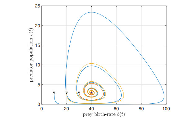
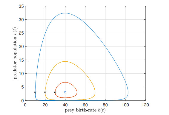
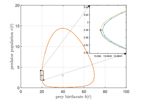
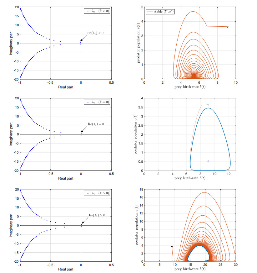
We study the impact of an age-dependent interaction in a structured predator-prey model. We present two approaches, the PDE (partial differential equation) and the renewal equation, highlighting the advantages of each one. We develop efficient numerical methods to compute the (un)stability of steady-states and the time-evolution of the interacting populations, in the form of oscillating orbits in the plane of prey birth-rate and predator population size. The asymptotic behavior when species interaction does not depend on age is completely determined through the age-profile and a predator-prey limit system of ODEs (ordinary differential equations). The appearance of a Hopf bifurcation is shown for a biologically meaningful age-dependent interaction, where the system transitions from a stable coexistence equilibrium to a collection of periodic orbits around it, and eventually to a stable limit cycle (isolated periodic orbit). Several explicit analytical solutions are used to test the accuracy of the proposed computational methods.
Citation: Jordi Ripoll, Jordi Font. Numerical approach to an age-structured Lotka-Volterra model[J]. Mathematical Biosciences and Engineering, 2023, 20(9): 15603-15622. doi: 10.3934/mbe.2023696
We study the impact of an age-dependent interaction in a structured predator-prey model. We present two approaches, the PDE (partial differential equation) and the renewal equation, highlighting the advantages of each one. We develop efficient numerical methods to compute the (un)stability of steady-states and the time-evolution of the interacting populations, in the form of oscillating orbits in the plane of prey birth-rate and predator population size. The asymptotic behavior when species interaction does not depend on age is completely determined through the age-profile and a predator-prey limit system of ODEs (ordinary differential equations). The appearance of a Hopf bifurcation is shown for a biologically meaningful age-dependent interaction, where the system transitions from a stable coexistence equilibrium to a collection of periodic orbits around it, and eventually to a stable limit cycle (isolated periodic orbit). Several explicit analytical solutions are used to test the accuracy of the proposed computational methods.

| [1] | M. Iannelli, F. Milner, The Basic Approach to Age-Structured Population Dynamics, Models, Methods and Numerics, Springer, Dordrecht, 2017. https://doi.org/10.1007/978-94-024-1146-1 |
| [2] | H. Thieme, Mathematics in population biology. Princeton Series in Theoretical and Computational Biology, Princeton University Press, Princeton, NJ, 2003. |
| [3] | H. Inaba, Age-structured population dynamics in demography and epidemiology, Springer, Berlin, 2017. https://doi.org/10.1007/978-981-10-0188-8 |
| [4] | H. Seno, A Primer on Population Dynamics Modeling: Basic Ideas for Mathematical Formulation, Springer, Singapore, 2022. https://doi.org/10.1007/978-981-19-6016-1 |
| [5] | G. F. Webb, Theory of Nonlinear Age-Dependent Population Dynamics, Marcel Dekker, New York, 1985. |
| [6] |
À. Calsina, J. Ripoll, Hopf bifurcation in a structured population model for the sexual phase of monogonont rotifers, J. Math. Biol.,45(2002), 22–36. https://doi.org/10.1007/s002850200147 doi: 10.1007/s002850200147

|
| [7] |
T. Kuniya, H. Inaba, Hopf bifurcation in a chronological age-structured SIR epidemic model with age-dependent infectivity, Math. Biosci. Eng., 20 (2023), 13036–13060. https://doi.org/10.3934/mbe.2023581 doi: 10.3934/mbe.2023581
|
| [8] |
Z. Liu, P. Magal, S. Ruan, Hopf bifurcation for non-densely defined Cauchy problems, Z. Angew. Math. Phys., 62 (2011), 191–222. https://doi.org/10.1007/s00033-010-0088-x doi: 10.1007/s00033-010-0088-x
|
| [9] | J. Chu, P. Magal, Hopf bifurcation for a size-structured model with resting phase, Discrete Contin. Dyn. Syst. - Ser. A, 2013, 33 (2013), 4891–4921. https://doi.org/10.3934/dcds.2013.33.4891 |
| [10] |
Z. Liu, H. Tang, P. Magal, Hopf bifurcation for a spatially and age structured population dynamics model, Discrete Contin. Dyn. Syst. - Ser. B, 20 (2015), 1735–1757. https://doi.org/10.3934/dcdsb.2015.20.1735 doi: 10.3934/dcdsb.2015.20.1735
|
| [11] |
J. Chu, A. Ducrot, P. Magal, Hopf bifurcation in a size-structured population dynamic model with random growth, J. Differ. Equat., 247 (2009), 956–1000. https://doi.org/10.1016/j.jde.2009.04.003 doi: 10.1016/j.jde.2009.04.003
|
| [12] |
S. Bentout, S. Djilali, A. Atangana, Bifurcation analysis of an age-structured prey–predator model with infection developed in prey, Math. Meth. Appl. Sci., 45 (2022), 1189–1208. https://doi.org/10.1002/mma.7846 doi: 10.1002/mma.7846
|
| [13] |
S. Bentout, S. Kumar, S. Djilali, Hopf bifurcation analysis in an age-structured heroin model, Eur. Phys. J. Plus, 136 (2021), 1–13. https://doi.org/10.1140/epjp/s13360-020-01001-7 doi: 10.1140/epjp/s13360-020-01001-7
|
| [14] | M. Iannelli, A. Pugliese, An Introduction to Mathematical Population Dynamics. Along the Trail of Volterra and Lotka; Springer, New York, NY, USA, 2014. https://doi.org/10.1007/978-3-319-03026-5 |
| [15] | N. Bacaër, A Short History of Mathematical Population Dynamics, Springer, London, UK, 2011. https://doi.org/10.1007/978-0-85729-115-8 |
| [16] | N. Bacaër, R. Bravo de la Parra, J. Ripoll, Breve Historia de los Modelos Matemáticos en Dinámica de Poblaciones, Cassini: Paris, France, 2021. (in Spanish) |
| [17] |
M. Gurtin, D. Levine, On predator-prey interactions with predation dependent on age of prey, Math. Biosci., 47 (1979), 207–219. https://doi.org/10.1016/0025-5564(79)90038-5 doi: 10.1016/0025-5564(79)90038-5
|
| [18] |
E. Venturino, Age-structured predator-prey models, Math. Modell., 5 (1984), 117–128. https://doi.org/10.1016/0270-0255(84)90020-4 doi: 10.1016/0270-0255(84)90020-4
|
| [19] |
A. Perasso, Q. Richard, Implication of age-structure on the dynamics of Lotka Volterra equations, Differ. Integr. Equations, 32 (2019), 91–120. https://doi.org/10.57262/die/1544497287 doi: 10.57262/die/1544497287
|
| [20] |
C. Barril, À. Calsina, O. Diekmann, J. Z. Farkas, On the formulation of size-structured consumer resource models (with special attention for the principle of linearized stability), Math. Models Methods Appl. Sci., 32 (2022), 1141–1191. https://doi.org/10.1142/S0218202522500269 doi: 10.1142/S0218202522500269
|
| [21] | D. Breda, S. Maset, R. Vermiglio, Stability of Linear Delay Differential Equations. A Numerical Approach with MATLAB. SpringerBriefs in Electrical and Computer Engineering. SpringerBriefs in Control, Automation and Robotics. Springer, New York, (2015). https://doi.org/10.1007/978-1-4939-2107-2 |
| [22] |
F. Scarabel, D. Breda, O. Diekmann, M. Gyllenberg, R. Vermiglio, Numerical Bifurcation Analysis of Physiologically Structured Population Models via Pseudospectral Approximation, Vietnam J. Math., 49 (2021), 37–67. https://doi.org/10.1007/s10013-020-00421-3 doi: 10.1007/s10013-020-00421-3
|
| [23] |
D. Breda, T. Kuniya, J. Ripoll, R. Vermiglio, Collocation of Next-Generation Operators for Computing the Basic Reproduction Number of Structured Populations, J. Sci. Comput., 85 (2020), 40. https://doi.org/10.1007/s10915-020-01339-1 doi: 10.1007/s10915-020-01339-1
|
| [24] |
D. Breda, F. Florian, J. Ripoll, R. Vermiglio, Efficient numerical computation of the basic reproduction number for structured populations, J. Comput. Appl. Math., 384 (2021), 113165. https://doi.org/10.1016/j.cam.2020.113165 doi: 10.1016/j.cam.2020.113165
|
| [25] |
A. Andò, S. De Reggi, D. Liessi, F. Scarabel, A pseudospectral method for investigating the stability of linear population models with two physiological structures, Math. Biosci. Eng., 20 (2023), 4493–4515. https://doi.org/10.3934/mbe.2023208 doi: 10.3934/mbe.2023208
|
| [26] |
D. Breda, R. Vermiglio, S. Maset, Computing the eigenvalues of Gurtin-MacCamy models with diffusion, IMA J. Numer. Anal., 32 (2012), 1030–1050. https://doi.org/10.1093/imanum/drr004 doi: 10.1093/imanum/drr004
|
| [27] |
D. Breda, C. Cusulin, M. Iannelli, S. Maset, R. Vermiglio, Stability analysis of age-structured population equations by pseudospectral differencing methods, J. Math. Biol., 54 (2007), 701–720. https://doi.org/10.1007/s00285-006-0064-4 doi: 10.1007/s00285-006-0064-4
|
| [28] |
D. Breda, M. Iannelli, S. Maset, R. Vermiglio, Stability analysis of the Gurtin-MacCamy model, SIAM J. Numer. Anal., 46 (2008), 980–995. https://doi.org/10.1137/070685658 doi: 10.1137/070685658
|
| [29] |
C. Barril, À. Calsina, J. Ripoll, A practical approach to $R_0$ in continuous-time ecological models, Math. Meth. Appl. Sci., 41 (2018), 8432–8445. https://doi.org/10.1002/mma.4673 doi: 10.1002/mma.4673
|
| [30] |
C. Barril, À. Calsina, S. Cuadrado, J. Ripoll, On the basic reproduction number in continuously structured populations, Math. Meth. Appl. Sci., 44 (2021), 799–812. https://doi.org/10.1002/mma.6787 doi: 10.1002/mma.6787
|
| [31] | R. Rudnicki, Mathematical modelling of population dynamics, volume 63 of Banach Center Publications, Polish Academy of Sciences Institute of Mathematics, Warsaw, 2004. |
| [32] |
M. Gyllenberg, G. F. Webb, Asynchronous exponential growth of semigroups of nonlinear operators, J. Math. Anal. Appl., 167 (1992), 443–467. https://doi.org/10.1016/0022-247X(92)90218-3 doi: 10.1016/0022-247X(92)90218-3
|
| [33] | K. J. Engel, R. Nagel, One-Parameter Semigroups for Linear Evolution Equations, no. 194 in Grad. Texts in Math., Springer, New York, 2000. |
| [34] |
O. Angulo, J. C. López-Marcos, M. A. López-Marcos, F. A. Milner, A numerical method for nonlinear age-structured population models with finite maximum age, J. Math. Anal. Appl., 361 (2010), 150–160. https://doi.org/10.1016/j.jmaa.2009.09.001 doi: 10.1016/j.jmaa.2009.09.001
|
| [35] | M. Martcheva, An Introduction to Mathematical Epidemiology, Springer, New York, 2015. https://doi.org/10.1007/978-1-4899-7612-3 |
Figures(5)

Jordi Ripoll, Jordi Font. Numerical approach to an age-structured Lotka-Volterra model[J]. Mathematical Biosciences and Engineering, 2023, 20(9): 15603-15622. doi: 10.3934/mbe.2023696


 DownLoad: