Scalable computational algorithms for geospatial COVID-19 spread using high performance computing

Sudhi Sharma; Victorita Dolean; Pierre Jolivet; Brandon Robinson; Jodi D. Edwards; Tetyana Kendzerska; Abhijit Sarkar; Sudhi Sharma; Victorita Dolean; Pierre Jolivet; Brandon Robinson; Jodi D. Edwards; Tetyana Kendzerska; Abhijit Sarkar

doi:10.3934/mbe.2023655

Mathematical Biosciences and Engineering

2023, Volume 20, Issue 8: 14634-14674. doi: 10.3934/mbe.2023655

Previous Article Next Article

Research article Special Issues

Scalable computational algorithms for geospatial COVID-19 spread using high performance computing

1.
Department of Civil and Environmental Engineering, Carleton University, Ottawa, Ontario, Canada
2.
Department of Mathematics and Statistics, University of Strathclyde, Glasgow, Scotland
3.
Laboratoire J.A. Dieudonné, CNRS, Université Côte d'Azur, Nice, France
4.
Sorbonne Université, CNRS, Paris, France
5.
School of Epidemiology and Public Health, University of Ottawa and University of Ottawa Heart Institute, Ottawa, Ontario, Canada
6.
ICES, Ottawa, Ontario, Canada
7.
The Ottawa Hospital Research Institute, Ottawa, Ontario, Canada
8.
Department of Medicine, Faculty of Medicine, Division of Respirology, University of Ottawa, Ottawa, Ontario, Canada

Academic Editor: Haralampos Hatzikirou

Received: 03 August 2022 Revised: 15 January 2023 Accepted: 21 February 2023 Published: 05 July 2023

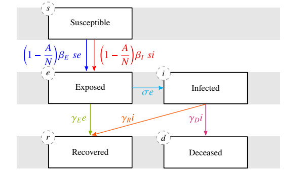
A nonlinear partial differential equation (PDE) based compartmental model of COVID-19 provides a continuous trace of infection over space and time. Finer resolutions in the spatial discretization, the inclusion of additional model compartments and model stratifications based on clinically relevant categories contribute to an increase in the number of unknowns to the order of millions. We adopt a parallel scalable solver that permits faster solutions for these high fidelity models. The solver combines domain decomposition and algebraic multigrid preconditioners at multiple levels to achieve the desired strong and weak scalabilities. As a numerical illustration of this general methodology, a five-compartment susceptible-exposed-infected-recovered-deceased (SEIRD) model of COVID-19 is used to demonstrate the scalability and effectiveness of the proposed solver for a large geographical domain (Southern Ontario). It is possible to predict the infections for a period of three months for a system size of 186 million (using 3200 processes) within 12 hours saving months of computational effort needed for the conventional solvers.

Keywords:

Citation: Sudhi Sharma, Victorita Dolean, Pierre Jolivet, Brandon Robinson, Jodi D. Edwards, Tetyana Kendzerska, Abhijit Sarkar. Scalable computational algorithms for geospatial COVID-19 spread using high performance computing[J]. Mathematical Biosciences and Engineering, 2023, 20(8): 14634-14674. doi: 10.3934/mbe.2023655

Related Papers:

[1]	Victor Zhenyu Guo . Almost primes in Piatetski-Shapiro sequences. AIMS Mathematics, 2021, 6(9): 9536-9546. doi: 10.3934/math.2021554
[2]	Yukai Shen . $k$ th powers in a generalization of Piatetski-Shapiro sequences. AIMS Mathematics, 2023, 8(9): 22411-22418. doi: 10.3934/math.20231143
[3]	Jinyun Qi, Zhefeng Xu . Almost primes in generalized Piatetski-Shapiro sequences. AIMS Mathematics, 2022, 7(8): 14154-14162. doi: 10.3934/math.2022780
[4]	Yanbo Song . On two sums related to the Lehmer problem over short intervals. AIMS Mathematics, 2021, 6(11): 11723-11732. doi: 10.3934/math.2021681
[5]	Xiaoqing Zhao, Yuan Yi . High-dimensional Lehmer problem on Beatty sequences. AIMS Mathematics, 2023, 8(6): 13492-13502. doi: 10.3934/math.2023684
[6]	Mingxuan Zhong, Tianping Zhang . Partitions into three generalized D. H. Lehmer numbers. AIMS Mathematics, 2024, 9(2): 4021-4031. doi: 10.3934/math.2024196
[7]	Bingzhou Chen, Jiagui Luo . On the Diophantine equations $x^2-Dy^2=-1$ and $x^2-Dy^2=4$ . AIMS Mathematics, 2019, 4(4): 1170-1180. doi: 10.3934/math.2019.4.1170
[8]	Rui Wang, Jiangtao Peng . On the inverse problems associated with subsequence sums of zero-sum free sequences over finite abelian groups Ⅱ. AIMS Mathematics, 2021, 6(2): 1706-1714. doi: 10.3934/math.2021101
[9]	Jinyan He, Jiagui Luo, Shuanglin Fei . On the exponential Diophantine equation $(a(a-l)m^{2}+1)^{x}+(alm^{2}-1)^{y} = (am)^{z}$ . AIMS Mathematics, 2022, 7(4): 7187-7198. doi: 10.3934/math.2022401
[10]	Baria A. Helmy, Amal S. Hassan, Ahmed K. El-Kholy, Rashad A. R. Bantan, Mohammed Elgarhy . Analysis of information measures using generalized type-Ⅰ hybrid censored data. AIMS Mathematics, 2023, 8(9): 20283-20304. doi: 10.3934/math.20231034

Abstract

1. Introduction

Let $q$ be an integer. For each integer $a$ with

$1 \leqslant a < q,\ \ (a, q) = 1,$

we know that ^[1] there exists one and only one $\bar{a}$ with

$1 \leqslant\bar{a} < q$

such that

$a \bar{a} \equiv 1(q).$

Define

$R(q): = \{a: 1 \leqslant a \leqslant q,(a, q) = 1,2 \nmid a+\bar{a}\},$

$r(q): = \# R(q).$

The work ^[2] posed the problem of investigating a nontrivial estimation for $r(q)$ when $q$ is an odd prime. Zhang ^[3,4] gave several asymptotic formulas for $r(q)$ , one of which is:

$r(q) = \frac{1}{2} \phi(q)+O\left(q^{\frac{1}{2}} d^{2}(q) \log ^{2} q\right),$

where $\phi(q)$ is the Euler function and $d(q)$ is the divisor function. Lu and Yi ^[5] studied a generalization of the Lehmer problem over short intervals. Let $n \geqslant 2$ be a fixed positive integer, $q \geqslant 3$ and $c$ be integers with

$(n c, q) = 1.$

They defined

$\begin{align*} r_n\left(\theta_1, \theta_2, c ; q\right) = \#\left\{(a, b) \in\left[1, \theta_1 q\right] \times\left[1, \theta_2 q\right] \mid a b \equiv c( \text{ mod } q), n \nmid a+b\right\}, \end{align*}$

where $0 < \theta_1, \theta_2 \leqslant 1$ , and obtained

$r_n\left(\theta_1, \theta_2, c ; q\right) = \left(1-\frac{1}{n}\right) \theta_1 \theta_2 \varphi(q)+O\left(q^{1 / 2} \tau^6(q) \log ^2 q\right),$

where the $O$ constant depends only on $n$ . In addition, Xi and Yi ^[6] considered generalized Lehmer problem over short intervals. Han and Liu ^[7] gave an upper bound estimation for another generalization of the Lehmer problem over incomplete interval.

Guo and Yi ^[8] also found the Lehmer problem has good distribution properties on Beatty sequences. For fixed real numbers $\alpha$ and $\beta$ , defined by

$\mathcal{B}_{\alpha, \beta}: = (\lfloor\alpha n+\beta\rfloor)_{n = 1}^{\infty}.$

Beatty sequences are linear sequences. Based on the results obtained, we conjecture the Lehmer problem also has good distribution properties in some non-linear sequences.

The Piatetski-Shapiro sequence is a non-linear sequence, defined by

$\mathbb{N}^c = \left\{\left\lfloor n^c\right\rfloor: n \in \mathbb{N}\right\},$

where $c \in \mathbb{R}$ is non-integer with $c > 1$ and $z \in \mathbb{R}$ . This sequence was first introduced by Piatetski-Shapiro ^[9] to study prime numbers in sequences of the form $\lfloor f(n)\rfloor$ , where $f(n)$ is a polynomial. A positive integer is called square-free if it is a product of distinct primes. The distribution of square-free numbers in the Piatetski-Shapiro sequence has been studied extensively. Stux ^[10] found that, as $x$ tends to infinity,

$\begin{align} \sum\limits_{\substack{n \leq x \\ \left\lfloor n^c\right\rfloor \text { is square-free }}} 1 = \left(\frac{6}{\pi^2}+o(1)\right) x, \quad \text { for }\ 1 < c < \frac{4}{3} . \end{align}$

(1.1)

In 1978, Rieger ^[11] improved the range to $1 < c < 3 / 2$ and obtained

$\frac{6 x}{\pi^2}+O\left(x^{(2 c+1) / 4+\varepsilon}\right), \quad \text { for }\ 1 < c < \frac{3}{2} \text {. }$

Considering the results obtained, we develop this problem by investigating

$R(c;q): = \mathop{\sum\limits_{\;\;n \in \mathbb{N}^c \cap R(q)\\n \text { is square-free } }} 1$

and range of $c$ when $q$ tends to infinity. By methods of exponential sum and Kloosterman sums and fairly detailed calculations, we get the following result, which is significant for understanding the distribution properties of the Lehmer problem.

Theorem 1.1. Let $q$ be an odd integer and large enough,

$\gamma : = 1/c \; \; \; \mathit{\text{and}}\; \; \; c \in (1, \frac{4}{3}),$

we obtain

$\begin{align} R(c;q) = &\frac{3}{\pi^{2}}\prod\limits_{p\mid q}(1+p^{-1})^{-1}q^{\gamma} \\&+O\left( \sum\limits_{p\mid q}(1-p^{-\frac{1}{2}}) ^{-1} q^{\gamma-\frac{1}{2}}\right)+O\left(q^{\frac{7}{13}\gamma+\frac{4}{13}}\prod\limits_{p\mid q}(1-p^{-\frac{1}{2}})^{-1}\log q\right)\\ &+O\left( q^{\frac{3}{4}}d^{3}(q)\log q \right)+O\left(q^{ \gamma -\frac{1}{6}} d^{2}(q)\log^3 q\right), \end{align}$

where the $O$ constant only depends on c.

This paper consists of three main sections. Introduction covers the origins and developments of the Lehmer problem, along with several interesting results. It also presents relevant findings related to the Piatetski-Shapiro sequences. The second section includes some definitions and lemmas throughout the paper. The third section outlines the calculation process, where we use additive characteristics to convert the congruence equations into exponential sum problems. We then employ the Kloosterman sums and exponential sums methods to derive an interesting asymptotic formula.

2. Preliminary lemmas

To complete the proof of the theorem, we need the following several definitions and lemmas.

In this paper, we denote by $\lfloor t\rfloor$ and $\{t\}$ the integral part and the fractional part of $t$ , respectively. As is customary, we put

$\mathbf{e}(t): = e^{2 \pi \mathbf{i} t} \quad \text {and} \quad\{t\}: = t-\lfloor t\rfloor.$

The notation $\|t\|$ is used to denote the distance from the real number $t$ to the nearest integer; that is,

$\|t\|: = \min\limits_{n \in \mathbb{Z}}|t-n|.$

And $\sum^{\prime}$ indicates that the variable summed over takes values coprime to the number $q$ . Throughout the paper, $\varepsilon$ always denotes an arbitrarily small positive constant, which may not be the same at different occurrences; the implied constants in symbols $O, \ll$ , and $\gg$ may depend (where obvious) on the parameters $c \text{ and } \varepsilon$ , but are absolute otherwise. For given functions $F$ and $G$ , the notations

$F \ll G,\ \ \ G \gg F\ \ \ \text{and}\; \; \; F = O(G)$

are all equivalent to the statement that the inequality

$|F| \leqslant \mathcal{C}|G|$

holds with some constant $\mathcal{C} > 0$ .

Lemma 2.1. Let $\mathbf{1}_{c}(m)$ denote the characteristic function of numbers in a Piatetski-Shapiro sequence, then

$\mathbf{1}_{c}(m) = \gamma m^{\gamma-1} +O(m^{\gamma-2}) + \psi \left(-(m+1)^{\gamma}\right) -\psi(-m^{\gamma})\nonumber ,$

where

$\psi(t) = t- \lfloor t \rfloor-\frac{1}{2} \ \ \ \mathit{\text{and}}\; \; \; \gamma = 1/c.$

Proof. Note that an integer $m$ has the form

$m = \lfloor n^c\rfloor$

for some integer $n$ if and only if

$m \leqslant n^{c} < m+1,\quad -(m+1)^{\gamma} < - n \leqslant -m^{\gamma}.$

$\begin{align} \mathbf{1}_{c}(m)& = \left\lfloor-m^{\gamma}\right\rfloor-\left\lfloor-(m+1)^{\gamma}\right\rfloor \\ & = -m^{\gamma} - \psi (-m^{\gamma}) +(m+1)^{\gamma}+\psi(-(m+1)^{\gamma})\\ & = \gamma m^{\gamma-1} +O(m^{\gamma-2})+ \psi\left (-(m+1)^{\gamma}\right) -\psi(-m^{\gamma}). \end{align}$

Thie completes the proof. □

Lemma 2.2. Let $H \geqslant 1$ be an integer, $a_h, b_h$ be real numbers, we have

$\left|\psi(t)-\sum\limits_{0 < |h| \leqslant H} a_h \mathbf{e}(t h)\right| \leqslant \sum\limits_{|h| \leqslant H} b_h \mathbf{e}(t h), \quad a_h \ll \frac{1}{|h|}, \quad b_h \ll \frac{1}{H}.$

Proof. In 1985, Vaaler showed how Beurling's function could be used to construct a trigonometric polynomial approximation to $\psi (x).$ For each positive integer $N$ , Vaaler's construction yields a trigonometric polynomial $\psi^*$ of degree $N$ which satisfies

$|\psi^*(x)-\psi(x)|\leq\frac1{2N+2}\sum\limits_{|n|\leq N}\left(1-\frac{|n|}{N+1}\right)\mathbf{e}(nx),$

where

$\begin{align*} \psi^*(x)& = -\mathop{\sum}_{1\leq|n|\leq N}(2\pi in)^{-1}\hat{J}_{N+1}(n)\mathbf{e}(nx), \\ H(z)& = \frac{\sin^2\pi z}{\pi^2}\left\{\sum\limits_{n = -\infty}^\infty\frac{\mathrm{sgn\; }(n)}{(z-n)^2}+\frac2z\right\},\quad J(z) = \frac12H^{\prime}(z),\\ H_N(z)& = \frac{\sin^2\pi z}{\pi^2}\left\{\sum\limits_{|n|\leq N}\frac{\mathrm{sgn\; }(n)}{(z-n)^2}+\frac2z\right\}, \quad J_N(z) = \frac12H_N^{\prime}(z), \end{align*}$

and $\mathrm{sgn\; }(n)$ is the sign of $n$ . The Fourier transform $\hat{J}(t)$ satisfies

$\begin{align} \hat{J}(t) = \begin{cases} 1 , & t = 0 ;\\ \pi t(1-|t|)\cot\pi t+|t|,& 0 < |t| < 1;\\ 0,& t\geq1.\end{cases} \end{align}$

To be short, we denote

$\begin{align*} a_h& = -(2\pi ih)^{-1}\hat{J}_{H+1}(h) \ll \frac{1}{|h|},\\ b_h& = \frac1{2H+2}\left(1-\frac{|h|}{H+1}\right)\ll \frac{1}{H}. \end{align*}$

There are more details in Appendix Theorem A.6. of ^[12]. □

Lemma 2.3. Denote

$\mathbf{Kl}(m,n;q) = \mathop{\sum\limits_{a = 1}^q \sum\limits_{b = 1}^q}_{a b \equiv 1( \bmod q)}\mathbf{e}\left(\frac{m a+n b}{q}\right),$

then

$\mathbf{Kl}(m,n;q) \ll(m, n, q)^{\frac{1}{2}} q^{\frac{1}{2}} d(q),$

where $(m, n, q)$ is the greatest common divisor of $m, n$ and $q$ and $d(q)$ is the number of positive divisors of $q$ .

Proof. The proof is given in ^[13]. □

Lemma 2.4. (Korobov ^[14]) Let $\alpha$ be a real number, $Q$ be an integer, and $P$ be a positive integer, then

$\left|\sum\limits_{x = Q+1}^{Q+P} \mathbf{e}(\alpha x)\right| \leqslant \min \left(P, \frac{1}{2\|\alpha\|}\right) .$

Lemma 2.5. (Karatsuba ^[15]) For any number $b$ , $U < 0$ , $K \geqslant 1$ , let

$a = \frac{s}{r}+\frac{\theta}{r^{2}}, \quad(r, s) = 1,\ \ \ r \geqslant 1,\ \ \ |\theta| \leqslant 1,$

then

$\sum\limits_{k \leqslant K} \min \left(U, \frac{1}{\|a k+b\|}\right) \ll\left(\frac{K}{r}+1\right)(U+r \log r).$

Lemma 2.6. Suppose $f$ is continuously differentiable, $f^{\prime}(n)$ is monotonic, and

$\left\|f^{\prime}(n)\right\| \geqslant \lambda_1 > 0$

on $I$ , then

$\sum\limits_{n \in I} \mathbf{e}\left(f(n)\right) \ll \lambda_1^{-1} .$

Proof. See [12, Theorem 2.1]. □

Lemma 2.7. Let $k$ be a positive integer, $k \geqslant 2$ . Suppose that $f(n)$ is a real-valued function with $k$ continuous derivatives on $[N, 2N],$ Further suppose that

$0 < F \leqslant f^{(k)}(n) \leqslant h F.$

Then

$\left|\sum\limits_{N < x \leqslant 2N} \mathbf{e}(f(n)) \right| \ll F^{\kappa} N^\lambda + F^{-1},$

where the implied constant is absolute.

Proof. See [12, Chapter 3]. □

3. Proof of theorem

By the definition of Mobius function

$\begin{align} \mu(n) = \begin{cases} (-1)^{\omega(n)} , & \forall p|n, p^2 \nmid n ,\\ 0,& \quad \exists p^2 |n ,\end{cases} \end{align}$

it is clear that $n$ is square-free if and only if

$\mu^{2}(n) = 1,$

where $\omega(n)$ is the number of prime divisor of $n$ . So

$\begin{align} R(c; q)& = \frac{1}{2} \mathop{{\sum}^{\prime}}_{n = 1}^{q} \left(1-(-1)^{n+\bar{n}}\right)\mu^{2}(n) \mathbf{1}_{c}(n)\\ & = \frac{1}{2}(R_{1}-R_{2}), \end{align}$

(3.1)

where

$\begin{align} R_{1} = \mathop{{\sum}^{\prime}}_{n = 1}^{q} \mu^{2}(n) \mathbf{1}_{c}(n) \end{align}$

and

$\begin{align} R_{2} = \mathop{{\sum}^{\prime}}_{n = 1}^{q} (-1)^{n+\bar{n}}\mu^{2}(n) \mathbf{1}_{c}(n). \end{align}$

3.1. Estimation of $R_{1}$

From Lemma 2.1, we have

$\begin{align} R_{1} & = \mathop{{\sum}^{\prime}}_{n = 1}^{q} \mu^{2}(n) \mathbf{1}_{c}(n) \\ & = \mathop{{\sum}^{\prime}}_{n = 1}^{q} \mu^{2}(n)\left( \gamma n^{\gamma-1} +O(n^{\gamma-2}) + \psi\left (-(n+1)^{\gamma}\right) -\psi(-n^{\gamma}) \right) \\ & = R_{11}+R_{12} , \end{align}$

(3.2)

where

$\begin{align} R_{11}&: = \mathop{{\sum}^{\prime}}_{n = 1}^{q} \mu^{2}(n)\left( \gamma n^{\gamma-1} +O(n^{\gamma-2}) \right)\\ & = \mathop{{\sum}^{\prime}}_{n = 1}^{q} \mu^{2}(n)\gamma n^{\gamma-1}+ O\left(\mathop{{\sum}^{\prime}}_{n = 1}^{q} \mu^{2}(n)n^{\gamma-2}\right) . \end{align}$

Let

$\mathcal{D} = \{d: p|d \Rightarrow p| q\}$

and $\lambda(n)$ is Liouville function. When $n \in R(q)$ ,

$\begin{align} \mu^{2}(n) = \begin{cases} \sum\limits_{dm = n,d\in \mathcal{D}} \lambda(d) \mu^{2}(m), &(n,q) = 1 ,\\ 0,& (n,q) > 1 .\end{cases} \end{align}$

(3.3)

We just consider the first term of $R_{11}$ . Applying Euler summuation ^[1],

$\begin{align} \mathop{{\sum}^{\prime}}_{n = 1}^{q} \mu^{2}(n)\gamma n^{\gamma-1} & = \mathop{\sum}_{n = 1}^{q} \mathop{\sum\limits_{dm = n }}_{d\in \mathcal{D}} \lambda(d) \mu^{2}(m) \gamma(dm)^{\gamma-1}\\ & = \sum\limits_{d\in \mathcal{D} } \lambda(d)d^{\gamma-1} \sum\limits_{m\leqslant\frac{q}{d}}\mu^{2}(m) \gamma m^{\gamma-1}\\ & = \sum\limits_{d\in \mathcal{D}} \lambda(d)d^{\gamma-1} \sum\limits_{m\leqslant\frac{q}{d}}\left(\sum\limits_{l^2\mid m}\mu (l)\right) \gamma m^{\gamma-1}\\ & = \sum\limits_{d\in \mathcal{D}} \lambda(d)d^{\gamma-1} \sum\limits_{l\leqslant(\frac{q}{d})^{\frac{1}{2}}}\mu (l)l^{2\gamma-2} \sum\limits_{m\leqslant\frac{q}{dl^2}}\gamma m^{\gamma-1}\\ & = \sum\limits_{d\in \mathcal{D}} \lambda(d)d^{\gamma-1} \sum\limits_{l\leqslant(\frac{q}{d})^{\frac{1}{2}}}\mu (l)l^{2\gamma-2}\left((\frac{q}{dl^2})^{\gamma}+O\left((\frac{q}{dl^2})^{\gamma-1}\right)\right) \\ & = q^{\gamma}\sum\limits_{d\in \mathcal{D}} \lambda(d)d^{-1} \sum\limits_{l\leqslant(\frac{q}{d})^{\frac{1}{2}}}\mu (l)l^{ -2} +O\left(\sum\limits_{d\in \mathcal{D}} \sum\limits_{l\leqslant(\frac{q}{d})^{\frac{1}{2}}} q^{\gamma-1}\right)\\ & = q^{\gamma}\sum\limits_{d\in \mathcal{D}} \lambda(d)d^{-1} \left(\sum\limits_{l}\mu (l)l^{ -2}+O\left((\frac{q}{d})^{-\frac{1}{2}}\right)\right) +O\left( \prod\limits_{p\mid q}(1-p^{-\frac{1}{2}}) ^{-1} q^{\gamma-\frac{1}{2}}\right)\\ & = \frac{6}{\pi^{2}}\prod\limits_{p\mid q}(1+p^{-1})^{-1}q^{\gamma} +O\left( \prod\limits_{p\mid q}(1-p^{-\frac{1}{2}}) ^{-1} q^{\gamma-\frac{1}{2}}\right), \end{align}$

thus

$\begin{align} R_{11} = \frac{6}{\pi^{2}}\prod\limits_{p\mid q}(1+p^{-1})^{-1}q^{\gamma} +O\left( \prod\limits_{p\mid q}(1-p^{-\frac{1}{2}}) ^{-1} q^{\gamma-\frac{1}{2}}\right). \end{align}$

(3.4)

For $R_{12}$ , by Lemma 2.2, we have

$\begin{align} R_{12}&: = \mathop{{\sum}^{\prime}}_{n = 1}^{q} \mu^{2}(n) \left(\psi\left(-(n+1)^{\gamma}\right)-\psi(-n^{\gamma})\right)\\ & = R_{121}+O(R_{122}), \end{align}$

(3.5)

where

$\begin{align} R_{121}: = \mathop{{\sum}^{\prime}}_{n = 1}^{q} \mu^{2}(n) \left(\sum\limits_{0 < |h|\leqslant H}a_{h}\left(\mathbf{e}\left(-(n+1)^{\gamma}h\right)-\mathbf{e}\left(-n^{\gamma}h\right)\right)\right) \end{align}$

and

$\begin{align} R_{122}: = \mathop{{\sum}^{\prime}}_{n = 1}^{q} \mu^{2}(n) \left(\sum\limits_{|h|\leqslant H}b_{h}\left(\mathbf{e}\left(-(n+1)^{\gamma}h\right)+\mathbf{e}\left(-n^{\gamma}h\right)\right)\right ). \end{align}$

Define

$f(t) = \mathbf{e}\left(\left((dt)^{\gamma}-(dt+1)^{\gamma}\right)h\right)-1,$

then

$\begin{align} f(t) &\ll\ |h| (dt)^{\gamma-1}, \\ \frac{\partial f(t)}{\partial t} &\ll |h| d^{\gamma-1}t^{\gamma-2}. \end{align}$

By Lemma 2.2 and Eq (3.3),

$\begin{align} R_{121} = &\sum\limits_{0 < |h|\leqslant H}a_{h} \sum\limits_{d\in \mathcal{D}} \lambda(d) \left(\sum\limits_{1 < m \leqslant \frac{q}{d}} \mu^{2}(m) \mathbf{e}\left(- (dm)^{\gamma}h\right) f(m)\right) \\ \ll& \sum\limits_{0 < |h|\leqslant H}|h|^{-1} \sum\limits_{d\in \mathcal{D}} \left|\int_{0}^{ \frac{q}{d}} f(t) \mathrm{d}\left(\sum\limits_{1 < m \leqslant t} \mu^{2}(m) \mathbf{e}\left(- (dm)^{\gamma}h\right)\right) \right|\\ \ll& \sum\limits_{0 < |h|\leqslant H}|h|^{-1} \sum\limits_{d\in \mathcal{D}} \left| f(\frac{q}{d}) \left(\sum\limits_{1 < m \leqslant \frac{q}{d}} \mu^{2}(m) \mathbf{e}\left(- (dm)^{\gamma}h\right)\right) \right|\\ &+\sum\limits_{0 < |h|\leqslant H}|h|^{-1} \sum\limits_{d\in \mathcal{D}} \left|\int_{0}^{ \frac{q}{d}} \frac{\partial f(t)}{\partial t} \sum\limits_{1 < m \leqslant t} \mu^{2}(m) \mathbf{e}\left(- (dm)^{\gamma}h\right)\mathrm{d}t \right|. \end{align}$

Let

$(\kappa,\lambda) = (\frac{1}{6},\frac{2}{3})$

be an exponential pair. Applying Lemma 2.7, it's easy to see

$\begin{align} \sum\limits_{1 < m \leqslant t} \mu^{2}(m) \mathbf{e}\left(- (dm)^{\gamma}h\right) = &\sum\limits_{m\leqslant t} \left(\sum\limits_{l^{2}\mid m}\mu (l)\right) \mathbf{e}\left(- (dm)^{\gamma}h\right) \\ \ll& \sum\limits_{l\leqslant t^{\frac{1}{2}}}\left| \sum\limits_{m\leqslant \frac{t}{l^{2}}}\mathbf{e}\left(- (dl^2m)^{\gamma}h\right)\right| \\ \ll&\sum\limits_{l\leqslant t^{\frac{1}{2}}} \log q \left(\left((dl^2)^{\gamma}|h|(\frac{t}{l^{2}})^{\gamma-1}\right)^{\frac{1}{6}}(\frac{t}{l^{2}})^{\frac{2}{3} }+\left((dl^2)^{\gamma}|h|(\frac{t}{l^{2}})^{\gamma-1}\right)^{-1} \right)\\ \ll& \log q \sum\limits_{l\leqslant t^{\frac{1}{2}}}\left((d^{\gamma}|h|)^{\frac{1}{6}}{t}^{\frac{1}{6}\gamma+\frac{1}{2}}l^{-1}+(d^{\gamma}|h|)^{-1}t^{1-\gamma }l^{-2}\right)\\ \ll& (d^{\gamma}|h|)^{\frac{1}{6}}{t}^{\frac{1}{6}\gamma+\frac{1}{2}} \log^2 q+(d^{\gamma}|h|)^{-1}t^{1-\gamma }\log q \\ \ll&(d^{\gamma}|h|)^{\frac{1}{6}}{t}^{\frac{1}{6}\gamma+\frac{1}{2}} \log^2 q, \end{align}$

thus

$\begin{align} R_{121}\ll& \sum\limits_{0 < |h|\leqslant H}|h|^{-1} \sum\limits_{d\in \mathcal{D}} |h|q^{\gamma-1}(d^{\gamma}|h|)^{\frac{1}{6}}{(\frac{q}{d})}^{\frac{1}{6}\gamma+\frac{1}{2}} \log^2 q \\ &+\sum\limits_{0 < |h|\leqslant H}|h|^{-1} \sum\limits_{d\in \mathcal{D}} \int_{0}^{ \frac{q}{d}} | h| d^{\gamma-1}t^{\gamma-2}(d^{\gamma}|h|)^{\frac{1}{6}}{t}^{\frac{1}{6}\gamma+\frac{1}{2}} \log^2 q \mathrm{d}t \\ \ll& \sum\limits_{0 < |h|\leqslant H}|h|^{\frac{1}{6}}\sum\limits_{d\in \mathcal{D}}d^{-\frac{1}{2}}q^{\frac{7}{6}\gamma-\frac{1}{2}} \log^2 q \\ &+\sum\limits_{0 < |h|\leqslant H}|h|^{\frac{1}{6}} \sum\limits_{d\in \mathcal{D}}d^{\frac{7}{6}\gamma-1}\log^2 q\int_{0}^{ \frac{q}{d}} t^{\frac{7}{6}\gamma-\frac{3}{2}} \mathrm{d}t\\ \ll& H^{\frac{7}{6}}\prod\limits_{p\mid q}(1-p^{-\frac{1}{2}})^{-1}q^{\frac{7}{6}\gamma-\frac{1}{2}}\log^2 q. \end{align}$

(3.6)

For $R_{122}$ , the contribution from $h \neq0$ can be bounded by similar methods of Eq (3.6). Taking

$H = q^{\frac{9}{13}-\frac{7}{13}\gamma} \geqslant 1,$

we obtain

$\begin{align} R_{122} & = b_{0} \mathop{{\sum}^{\prime}}_{n = 1}^{q} \mu^{2}(n)+\sum\limits_{0 < |h|\leqslant H}b_{h} \mathop{{\sum}^{\prime}}_{n = 1}^{q} \mu^{2}(n) \left(e\left(-(n+1)^{\gamma}h\right)+e\left(-n^{\gamma}h\right)\right) \\ &\ll H^{-1}q + H^{\frac{7}{6}}\prod\limits_{p\mid q}(1-p^{-\frac{1}{2}})^{-1}q^{\frac{7}{6}\gamma-\frac{1}{2}}\log q \\ &\ll q^{\frac{7}{13}\gamma+\frac{4}{13}}\prod\limits_{p\mid q}(1-p^{-\frac{1}{2}})^{-1}\log^2 q. \end{align}$

(3.7)

It follows from Eqs ( $3.5$ )–( $3.7$ ),

$\begin{align} R_{12} \ll q^{\frac{7}{13}\gamma+\frac{4}{13}}\prod\limits_{p\mid q}(1-p^{-\frac{1}{2}})^{-1}\log^2 q . \end{align}$

Hence

$\begin{align} R_{1} = \frac{6}{\pi^{2}}\prod\limits_{p\mid q}(1+p^{-1})^{-1}q^{\gamma} +O\left( \sum\limits_{p\mid q}(1-p^{-\frac{1}{2}}) ^{-1} q^{\gamma-\frac{1}{2}}\right)+O\left(q^{\frac{7}{13}\gamma+\frac{4}{13}}\prod\limits_{p\mid q}(1-p^{-\frac{1}{2}})^{-1}\log^2 q\right). \end{align}$

(3.8)

3.2. Estimation of $R_{2}$

Similarly,

$\begin{align} R_{2} = & \mathop{{\sum}^{\prime}}_{n = 1}^{q} (-1)^{n+\bar{n}} \mu^{2}(n) \mathbf{1}_{c}(n) \\ = & RP_{21}+RP_{22} , \end{align}$

(3.9)

where

$\begin{align} R_{21} = \mathop{{\sum}^{\prime}}_{n = 1}^{q}(-1)^{n+\bar{n}} \mu^{2}(n)\left( \gamma n^{\gamma-1} +O(n^{\gamma-2}) \right) \end{align}$

and

$\begin{align} R_{22} = \mathop{{\sum}^{\prime}}_{n = 1}^{q}(-1)^{n+\bar{n}} \mu^{2}(n)\left(\psi\left(-(n+1)^{\gamma}\right)-\psi(-n^{\gamma})\right). \end{align}$

We also just consider the first term of $R_{21}$ .

$\begin{align} \mathop{{\sum}^{\prime}}_{n = 1}^{q}(-1)^{n+\bar{n}} \mu^{2}(n) \gamma n^{\gamma-1} = &\mathop{{\sum}^{\prime}}_{n = 1}^{q} (-1)^{n+\bar{n}}\left( \sum\limits_{d^{2}\mid n} \mu(d) \right) \gamma n^{\gamma-1} \\ = &\mathop{{\sum}^{\prime}}_{n = 1}^{q} (-1)^{n+\bar{n}} \mathop{\sum\limits_{d^{2}\mid n}}_{d \leqslant q^{\frac{1}{4} }} \mu(d) \gamma n^{\gamma-1}+\mathop{{\sum}^{\prime}}_{n = 1}^{q} (-1)^{n+\bar{n}} \mathop{\sum\limits_{d^{2}\mid n}}_{q^{\frac{1}{4} } < d \leqslant q^{\frac{1}{2}} } \mu(d) \gamma n^{\gamma-1}. \end{align}$

(3.10)

It is easy to see

$\begin{align} \mathop{{\sum}^{\prime}}_{n = 1}^{q} (-1)^{n+\bar{n}} \mathop{\sum\limits_{d^{2}\mid n}}_{q^{\frac{1}{4} } < d \leqslant q^{\frac{1}{2}} } \mu(d) \gamma n^{\gamma-1} \ll \mathop{{\sum}^{\prime}}_{n = 1}^{q} \mathop{\sum\limits_{d^{2}\mid n}}_{q^{\frac{1}{4} } < d \leqslant q^{\frac{1}{2}} } \gamma n^{\gamma-1} \ll q^{\gamma-\frac{1}{4} }. \end{align}$

(3.11)

Since for integers $m$ and $a$ , one has

$\frac{1}{q}\sum\limits_{s = 1}^{q}\mathbf{e}(\frac{s(m-a)}{q}) = \begin{cases} 1, &m \equiv a (\text{ mod } q);\\ 0, &m \not \equiv a (\text{ mod } q).\end{cases}$

This gives

$\begin{align} \mathop{{\sum}^{\prime}}_{n = 1}^{q} (-1)^{n+\bar{n}} \mathop{\sum\limits_{d^{2}\mid n}}_{d \leqslant q^{\frac{1}{4} }} \mu(d) \gamma n^{\gamma-1} = &\mathop{\sum\limits_{n = 1}^{q} \sum\limits_{m = 1}^{q} }_{nm \equiv 1 (\bmod q)} (-1)^{n+m} \mathop{\sum\limits_{d^{2}\mid n}}_{d \leqslant q^{\frac{1}{4} }} \mu(d) \gamma n^{\gamma-1} \mathop{\sum\limits_{a = 1}^{q-1}}_{a = m } \mathop{\sum\limits_{b = 1}^{q-1}}_{b = n } 1\\ = &\mathop{\sum\limits_{n = 1}^{q} \sum\limits_{m = 1}^{q} }_{nm \equiv 1 (\bmod q)} \mathop{\sum\limits_{a = 1}^{q-1}}_{a = m } \mathop{\sum\limits_{b = 1}^{q-1}}_{b = n } (-1)^{a+b} \mathop{\sum\limits_{d^{2}\mid b}}_{d \leqslant q^{\frac{1}{4} }} \mu(d) \gamma b^{\gamma-1} \\ = & \mathop{\sum\limits_{n = 1}^{q} \sum\limits_{m = 1}^{q} }_{nm \equiv 1 (\bmod q)} \mathop{\sum\limits_{a = 1}^{q-1}}_{a \equiv m (\bmod q) } \mathop{\sum\limits_{b = 1}^{q-1}}_{b \equiv n (\bmod q) }(-1)^{a+b}\mathop{\sum\limits_{d^{2}\mid b}}_{d \leqslant q^{\frac{1}{4} }} \mu(d) \gamma b^{\gamma-1} \\ = & \mathop{\sum\limits_{n = 1}^{q} \sum\limits_{m = 1}^{q} }_{nm \equiv 1 (\bmod q)} \sum\limits_{a = 1}^{q-1}\sum\limits_{b = 1}^{q-1}(-1)^{a+b}\mathop{\sum\limits_{d^{2}\mid b}}_{d \leqslant q^{\frac{1}{4} }} \mu(d) \gamma b^{\gamma-1} \\ &\times\left(\frac{1}{q}\sum\limits_{s = 1}^{q}\mathbf{e}(\frac{s(m-a)}{q}) \right)\left(\frac{1}{q}\sum\limits_{t = 1}^{q}\mathbf{e}(\frac{t(n-b)}{q})\right) \\ = &\frac{1}{q^{2}}\sum\limits_{s = 1}^{q}\sum\limits_{t = 1}^{q} \left( \mathop{\sum}_{nm \equiv 1 (\bmod q)} \mathbf{e}(\frac{sm+tn}{q}) \right)\\ &\times\left(\sum\limits_{a = 1}^{q-1}(-1)^{a}\mathbf{e}(-\frac{sa}{q})\right)\left(\sum\limits_{b = 1}^{q-1}(-1)^{b}\mathbf{e}(-\frac{tb}{q})\mathop{\sum\limits_{d^{2}\mid b}}_{d \leqslant q^{\frac{1}{4} }} \mu(d) \gamma b^{\gamma-1} \right ). \end{align}$

(3.12)

From Lemma 2.3,

$\begin{align} \mathop{\sum}_{nm \equiv 1 (\bmod q)} \mathbf{e}(\frac{sm+tn}{q}) = \mathbf{Kl}(s,t;q) \ll(s, t, q)^{\frac{1}{2}} q^{\frac{1}{2}} d(q) . \end{align}$

(3.13)

Note the estimate

$\begin{align} \left|\sum\limits_{a = 1}^{q-1}(-1)^{a}\mathbf{e}(-\frac{sa}{q}) \right| \ll\frac{1}{\left|e(\frac{1}{2}-\frac{s}{q})-1\right|}\ll\frac{1}{|\cos \frac{s}{q}\pi |} \end{align}$

(3.14)

holds. By Abel summation and Lemma 2.4, we have

$\begin{align} \sum\limits_{b = 1}^{q-1}(-1)^{b}\mathbf{e}(-\frac{tb}{q})\mathop{\sum\limits_{d^{2}\mid b}}_{d \leqslant q^{\frac{1}{4}}} \mu(d) \gamma b^{\gamma-1} = &\sum\limits_{d \leqslant q^{\frac{1}{4}}} \mu(d)\sum\limits_{b = 1}^{\lfloor\frac{q-1}{d^2}\rfloor}(-1)^{d^{2}b}\mathbf{e}(-\frac{td^{2}b}{q}) \gamma (d^2b)^{\gamma-1} \\ \ll&\sum\limits_{d \leqslant q^{\frac{1}{4}}} d^{2(\gamma-1)}\left|\sum\limits_{b = 1}^{\lfloor\frac{q-1}{d^2}\rfloor}(-1)^{d^{2}b}\mathbf{e}(-\frac{td^{2}b}{q}) \gamma b^{\gamma-1}\right| \\ \ll& \sum\limits_{d \leqslant q^{\frac{1}{4}}} d^{2(\gamma-1)}\gamma(\frac{q}{d^2})^{\gamma-1} \max\limits_{1 \leqslant \beta \leqslant \lfloor\frac{q-1}{d^2}\rfloor }\left| \sum\limits_{b = 1}^{\beta }(-1)^{d^{2}b}\mathbf{e}(-\frac{td^{2}b}{q}) \right| \\ \ll& \mathop{\sum\limits_{d \leqslant q^{\frac{1}{4}}}}_{2 \mid d}\gamma q^{ \gamma-1 }\max\limits_{1 \leqslant \beta \leqslant \lfloor\frac{q-1}{d^2}\rfloor }\left| \sum\limits_{b = 1}^{ \beta} \mathbf{e}(-\frac{td^{2}b}{q}) \right| \\ & +\mathop{\sum\limits_{d \leqslant q^{\frac{1}{4}}}}_{2 \nmid d} \gamma q^{ \gamma-1 }\max\limits_{1 \leqslant \beta \leqslant \lfloor\frac{q-1}{d^2}\rfloor }\left| \sum\limits_{b = 1}^{\beta }(-1)^{ b}\mathbf{e}(-\frac{td^{2}b}{q}) \right| \\ \ll& \mathop{\sum\limits_{d \leqslant q^{\frac{1}{4} }}}_{2 \mid d}q^{ \gamma-1 }\min\left( \lfloor\frac{q-1}{d^2}\rfloor,\frac{1}{2\|\frac{d^{2}}{q}t \|} \right)+\mathop{\sum\limits_{d \leqslant q^{\frac{1}{4} }}}_{2 \nmid d}q^{ \gamma-1 }\min\left( \lfloor\frac{q-1}{d^2}\rfloor,\frac{1}{2\|\frac{1}{2}-\frac{d^{2}}{q}t \|} \right) . \end{align}$

(3.15)

To be short, combining Eqs (3.13)–(3.15), we denote

$\begin{align} R_{211}: = &q^{-2}\sum\limits_{s = 1}^{q}\sum\limits_{t = 1}^{q}(s,t,q)^{\frac{1}{2}}d(q)q^{\frac{1}{2}}\frac{1}{|\cos\frac{s}{q}\pi|} \mathop{\sum\limits_{d \leqslant q^{\frac{1}{4} }}}_{2 \mid d}q^{ \gamma-1 }\min\left( \lfloor\frac{q-1}{d^2}\rfloor,\frac{1}{2\|\frac{d^{2}}{q}t \|} \right)\\ \ll& q^{ \gamma-3}\sum\limits_{s = 1}^{q}\sum\limits_{t = 1}^{q}(s,t,q)^{\frac{1}{2}}d(q)q^{\frac{1}{2}}\frac{1}{|\cos\frac{s}{q}\pi|} \sum\limits_{d \leqslant q^{\frac{1}{4} }} \min\left( \frac{q-1}{d^2},\frac{1}{2\|\frac{d^{2}}{q}t \|} \right)\\ \ll& q^{\gamma-3}\sum\limits_{u\mid q}u^{\frac{1}{2}} d(q)q^{\frac{1}{2}}\sum\limits_{s = 1}^{\frac{q}{u}}\frac{1}{|\cos\frac{su}{q}\pi|} \sum\limits_{d \leqslant q^{\frac{1}{4} }} \sum\limits_{t = 1}^{\frac{q}{u}}\min\left( \frac{q-1}{d^2},\frac{1}{2\|\frac{d^{2}}{\frac{q}{u}}t \|} \right) \end{align}$

and

$R_{212}: = q^{-2}\sum\limits_{s = 1}^{q}\sum\limits_{t = 1}^{q}(s,t,q)^{\frac{1}{2}}d(q)q^{\frac{1}{2}}\frac{1}{|\cos\frac{s}{q}\pi|} \mathop{\sum\limits_{d \leqslant q^{\frac{1}{4} }}}_{2 \nmid d}q^{ \gamma-1 }\min\left( \lfloor\frac{q-1}{d^2}\rfloor,\frac{1}{2\|\frac{1}{2}-\frac{d^{2}}{q}t \|} \right).\nonumber$

Let

$(d^{2},\frac{q}{u}) = r,\ \ \ (\frac{d^{2}}{r},\frac{q}{ur}) = 1,$

making use of Lemma 2.5, we have

$\sum\limits_{t = 1}^{\frac{q}{u}}\min\left( \frac{q-1}{d^2},\frac{1}{2\|\frac{d^{2}}{\frac{q}{u}}t \|} \right)\ll (\frac{\frac{q}{u}}{\frac{q}{ur}}+1)(\frac{q-1}{d^2}+\frac{q}{ur}\log q) \ll \frac{qr}{d^2}+ \frac{q }{u} \log q.$

Insert it to $R_{211}$ , then

$\begin{align} R_{211}\ll& q^{\gamma-3}\sum\limits_{u\mid q}u^{\frac{1}{2}} d(q)q^{\frac{1}{2}}\sum\limits_{s = 1}^{\frac{q}{u}}\frac{1}{|1-2 \frac{su}{q} |} \sum\limits_{d \leqslant q^{\frac{1}{4} }}\sum\limits_{(d^{2},\frac{q}{u}) = r}( \frac{qr}{d^2}+ \frac{q }{u} \log q)\\ \ll&q^{\gamma-3}\sum\limits_{u\mid q}u^{\frac{1}{2}} d(q)q^{\frac{1}{2}}\frac{q}{u}\log q\sum\limits_{d \leqslant q^{\frac{1}{4} }}\mathop{\sum\limits_{r |d^{2}}}_{r|\frac{q}{u} }( \frac{qr}{d^2}+ \frac{q }{u} \log q) \\ \ll&q^{\gamma-3}\sum\limits_{u\mid q}u^{\frac{1}{2}} d(q)q^{\frac{1}{2}}\frac{q}{u}\log q \sum\limits_{r |\frac{q}{u}}\sum\limits_{d \leqslant \frac{q^{\frac{1}{4} }}{r^{\frac{1}{2}}} }( \frac{q }{d^2}+ \frac{q }{u} \log q) \\ \ll&q^{\gamma-3}\sum\limits_{u\mid q}u^{\frac{1}{2}} d(q)q^{\frac{1}{2}}\frac{q}{u}\log q \left(qd(q)+\frac{q^{\frac{5}{4} }}{u}d(q)\log q\right)\\ \ll& q^{\gamma- \frac{1}{4} }d^{3}(q) \log^3 q. \end{align}$

By the same method of $R_{211}$ ,

$\begin{align} R_{212}\ll q^{\gamma- \frac{1}{4}}d^{3}(q) \log^3 q. \end{align}$

Following from Eqs (3.10) and (3.11), estimations of $R_{211}$ and $R_{212}$ ,

$\begin{align} R_{21}\ll q^{\gamma- \frac{1}{4}}+ RP_{211}+RP_{212}\ll q^{ \gamma- \frac{1}{4}}d^{3}(q) \log^3 q. \end{align}$

(3.16)

By the similar method of $R_{12}$ and $R_{21}$ ,

$\begin{align} R_{22} = R_{221}+O(R_{222}), \end{align}$

(3.17)

where

$\begin{align} R_{221}: = &\mathop{{\sum}^{\prime}}_{n = 1}^{q} (-1)^{n+\bar{n}} \mu^{2}(n)\left( \sum\limits_{0 < |h|\leqslant H}a_{h} \left(\mathbf{e}\left(-(n+1)^{\gamma}h\right)-\mathbf{e}(-n^{\gamma}h)\right)\right) \end{align}$

and

$\begin{align} R_{222}: = &\mathop{{\sum}^{\prime}}_{n = 1}^{q} (-1)^{n+\bar{n}} \mu^{2}(n)\left( \sum\limits_{ |h|\leqslant H}b_{h} \left(\mathbf{e}\left(-(n+1)^{\gamma}h\right)+\mathbf{e}(-n^{\gamma}h)\right)\right). \end{align}$

It is obvious that

$\begin{align} R_{221} = &\mathop{{\sum}^{\prime}}_{n = 1}^{q} (-1)^{n+\bar{n}}\left(\sum\limits_{d^{2} \mid n}\mu(d)\right)\left( \sum\limits_{0 < |h|\leqslant H}a_{h} \left(\mathbf{e}\left(-(n+1)^{\gamma}h\right)-\mathbf{e}(-n^{\gamma}h)\right)\right) \\ = &\mathop{{\sum}^{\prime}}_{n = 1}^{q} (-1)^{n+\bar{n}} \mathop{\sum\limits_{d^{2} \mid n}}_{d \leqslant q^{\frac{1}{6}}}\mu(d) \left( \sum\limits_{0 < |h|\leqslant H}a_{h} \left(\mathbf{e}\left(-(n+1)^{\gamma}h\right)-\mathbf{e}(-n^{\gamma}h)\right)\right) \\ & +\mathop{{\sum}^{\prime}}_{n = 1}^{q} (-1)^{n+\bar{n}} \mathop{\sum\limits_{d^{2} \mid n}}_{q^{\frac{1}{6}} < d \leqslant q^{\frac{1}{2}} }\mu(d) \left( \sum\limits_{0 < |h|\leqslant H}a_{h} \left(\mathbf{e}\left(-(n+1)^{\gamma}h\right)-\mathbf{e}(-n^{\gamma}h)\right)\right). \end{align}$

(3.18)

From the estimate

$\mathbf{e}\left(n^{\gamma}h-(n+1)^{\gamma}h\right)-1 \ll ( n^{\gamma} -(n+1)^{\gamma})h \ll \gamma n^{\gamma -1} h,$

by partial summation,

$\begin{align} &\mathop{{\sum}^{\prime}}_{n = 1}^{q} (-1)^{n+\bar{n}} \mathop{\sum\limits_{d^{2} \mid n}}_{q^{\frac{1}{6}} < d \leqslant q^{\frac{1}{2}} }\mu(d) \left( \sum\limits_{0 < |h|\leqslant H}a_{h} \left(\mathbf{e}\left(-(n+1)^{\gamma}h\right)-\mathbf{e}(-n^{\gamma}h)\right)\right) \\ &\ll\mathop{{\sum}^{\prime}}_{n = 1}^{q} \mathop{\sum\limits_{d^{2} \mid n}}_{q^{\frac{1}{6}} < d \leqslant q^{\frac{1}{2}} } \left| \sum\limits_{0 < |h|\leqslant H}a_{h} \mathbf{e}(-n^{\gamma}h) \left(\mathbf{e}\left(n^{\gamma}h-(n+1)^{\gamma}h\right)-1\right)\right| \\ &\ll\mathop{{\sum}^{\prime}}_{n = 1}^{q} \mathop{\sum\limits_{d^{2} \mid n}}_{q^{\frac{1}{6}} < d \leqslant q^{\frac{1}{2}} } \gamma n^{\gamma-1}H \log H \\ & \ll q^{\gamma-\frac{1}{6}}H \log H . \end{align}$

(3.19)

For another term of $R_{221}$ ,

$\begin{align} &\mathop{{\sum}^{\prime}}_{n = 1}^{q} (-1)^{n+\bar{n}} \mathop{\sum\limits_{d^{2} \mid n}}_{d \leqslant q^{\frac{1}{6}} }\mu(d) \left( \sum\limits_{0 < |h|\leqslant H}a_{h} \left(\mathbf{e}\left(-(n+1)^{\gamma}h\right)-\mathbf{e}(-n^{\gamma}h)\right)\right)\\ & = \mathop{{\sum}^{\prime}}_{n = 1}^{q} (-1)^{n+\bar{n}} \mathop{\sum\limits_{d^{2} \mid n}}_{d \leqslant q^{\frac{1}{6}} }\mu(d) \left( \sum\limits_{0 < |h|\leqslant H}a_{h} \left(\mathbf{e}\left(-(n+1)^{\gamma}h\right)-\mathbf{e}(-n^{\gamma}h)\right)\right) \\ &\quad\times \left(\frac{1}{q}\sum\limits_{a = 1}^{q}\sum\limits_{s = 1}^{q}\mathbf{e}(\frac{s(m-a)}{q}) \right)\left(\frac{1}{q}\sum\limits_{b = 1}^{q}\sum\limits_{t = 1}^{q}\mathbf{e}(\frac{t(n-b)}{q})\right) \\ & = \frac{1}{q^{2}}\sum\limits_{s = 1}^{q}\sum\limits_{t = 1}^{q} \left( \mathop{\sum}_{nm \equiv 1 (\bmod q)} \mathbf{e}(\frac{sm+tn}{q}) \right)\left(\sum\limits_{a = 1}^{q-1}(-1)^{a}\mathbf{e}(-\frac{sa}{q})\right)\\ &\quad\times \left(\sum\limits_{b = 1}^{q-1}(-1)^{b}\mathbf{e}(-\frac{tb}{q}) \mathop{\sum\limits_{d^{2} \mid b}}_{d \leqslant q^{\frac{1}{6} } }\mu(d) \sum\limits_{0 < |h|\leqslant H}a_{h} \left(\mathbf{e}\left(-(b+1)^{\gamma}h\right)-\mathbf{e}(-b^{\gamma}h)\right) \right ). \end{align}$

(3.20)

We just need to give an estimation of the last part in (3.20). Similarly, let

$g (x) = \mathbf{e}\left(\left((d^{2}x)^{\gamma}-(d^{2}x+1)^{\gamma}\right)h \right)-1,$

then

$\begin{align} g (x) &\ll\ |h| (d^2x)^{\gamma-1}, \\ \frac{\partial g(x)}{\partial x} &\ll |h| d^{2\gamma-2}x^{\gamma-2}. \end{align}$

By partial summation,

$\begin{align} &\sum\limits_{b = 1}^{q-1}(-1)^{b}\mathbf{e}(-\frac{tb}{q}) \mathop{\sum\limits_{d^{2} \mid b}}_{d \leqslant q^{\frac{1}{6} } }\mu(d) \sum\limits_{0 < |h|\leqslant H}a_{h} \left(\mathbf{e}\left(-(b+1)^{\gamma}h\right)-\mathbf{e}(-b^{\gamma}h)\right) \\ & = \sum\limits_{0 < |h|\leqslant H}a_{h} \sum\limits_{d \leqslant q^{ \frac{1}{6} }}\mu(d)\sum\limits_{1 \leqslant b \leqslant \lfloor\frac{q-1}{d^2}\rfloor} \mathbf{e}\left((\frac{d^{2}}{2}-\frac{td^{2}}{q})b-(d^{2}b)^{\gamma}h\right)g(b), \\ & \ll\sum\limits_{0 < |h|\leqslant H}|h|^{-1} \sum\limits_{d \leqslant q^{ \frac{1}{6} }} \left|\int_{ 1}^{ \lfloor\frac{q-1}{d^2}\rfloor} g(x) \mathrm{d}\left(\sum\limits_{1 < b \leqslant x} \mathbf{e}\left((\frac{d^{2}}{2}-\frac{td^{2}}{q})b-(d^{2}b)^{\gamma}h\right) \right) \right|\\ & \ll\sum\limits_{0 < |h|\leqslant H}|h|^{-1} \sum\limits_{d \leqslant q^{ \frac{1}{6} }} \left|g( \lfloor\frac{q-1}{d^2}\rfloor) \sum\limits_{ 1 \leqslant b \leqslant \lfloor\frac{q-1}{d^2}\rfloor} \mathbf{e}\left((\frac{d^{2}}{2}-\frac{td^{2}}{q})b-(d^{2}b)^{\gamma}h\right)\right|\\ &\quad +\sum\limits_{0 < |h|\leqslant H}|h|^{-1} \sum\limits_{d \leqslant q^{ \frac{1}{6} }} \left|\int_{ 1}^{ \lfloor\frac{q-1}{d^2}\rfloor}\frac{\partial g(x)}{\partial x} \sum\limits_{ 1 \leqslant b \leqslant x} \mathbf{e}\left((\frac{d^{2}}{2}-\frac{td^{2}}{q})b-(d^{2}b)^{\gamma}h\right) \mathrm{d}x\right|, \end{align}$

where

$g( \lfloor\frac{q-1}{d^2}\rfloor) \ll |h|q^{\gamma-1}$

and

$\begin{align} &\sum\limits_{ 1 \leqslant b \leqslant \lfloor\frac{q-1}{d^2}\rfloor} \mathbf{e}\left((\frac{d^{2}}{2}-\frac{td^{2}}{q})b-(d^{2}b)^{\gamma}h\right) \\ & = \sum\limits_{ 1 \leqslant b \leqslant q^{\frac{1}{6}} } \mathbf{e}\left((\frac{d^{2}}{2}-\frac{td^{2}}{q})b-(d^{2}b)^{\gamma}h\right)+\sum\limits_{ q^{\frac{1}{6}} < b \leqslant \lfloor\frac{q-1}{d^2}\rfloor} \mathbf{e}\left((\frac{d^{2}}{2}-\frac{td^{2}}{q})b-(d^{2}b)^{\gamma}h\right). \end{align}$

It is obvious that

$\begin{align} \sum\limits_{ 1 \leqslant b \leqslant q^{\frac{1}{6}} } \mathbf{e}\left((\frac{d^{2}}{2}-\frac{td^{2}}{q})b-(d^{2}b)^{\gamma}h\right)\ll q^{\frac{1}{6}}. \end{align}$

Suppose $q$ be large enough and for $b > q^{\frac{1}{6}}$ , when $2 \nmid d$ or $q \nmid td^2$ ,

$\left\| (\frac{d^{2}}{2}-\frac{td^{2}}{q})-\gamma d^{2\gamma}b^{\gamma-1}h\right\|^{-1} \geqslant \frac{1}{2} \left\| (\frac{1}{2}-\frac{t }{q})d^{2}\right\|^{-1} > 0,$

and applying Lemma 2.6, we have

$\begin{align} \sum\limits_{q^{\frac{1}{6}} < b \leqslant \lfloor\frac{q-1}{d^2}\rfloor} \mathbf{e}\left((\frac{d^{2}}{2}-\frac{td^{2}}{q})b-(d^{2}b)^{\gamma}h\right) \ll& \left\| (\frac{d^{2}}{2}-\frac{td^{2}}{q})-\gamma d^{2\gamma}b^{\gamma-1}h\right\|^{-1} \\ \ll& \left\| (\frac{1}{2}-\frac{t }{q})d^{2}\right\|^{-1} . \end{align}$

$\sum\limits_{ 1 \leqslant b \leqslant \lfloor\frac{q-1}{d^2}\rfloor} \mathbf{e}\left((\frac{d^{2}}{2}-\frac{td^{2}}{q})b-(d^{2}b)^{\gamma}h\right) \ll \begin{cases} q^{\frac{1}{6}}+ \left\| (\frac{1}{2}-\frac{t }{q})d^{2}\right\|^{-1} , & 2 \nmid d \text{ or } q \nmid td^2;\\ \frac{q}{d^2}, & 2 \mid d \text{ and } q \mid td^2 ;\end{cases}$

which means

We denote

$\begin{align} T(c)&: = \sum\limits_{d\leqslant q^{\frac{1}{6} }} \# \left\{ (\frac{q}{u}-2t)d^{2} \equiv c (\bmod 2\frac{q}{u}), t\leqslant \frac{q}{u}\right\} \\ &\ll \sum\limits_{d\leqslant q^{\frac{1}{6} }} (\frac{q}{u}, d^{2}) \\ &\ll q^{\frac{1}{3} }d(q), \end{align}$

thus,

$\begin{align} &\mathop{{\sum}^{\prime}}_{n = 1}^{q} (-1)^{n+\bar{n}} \mathop{\sum\limits_{d^{2} \mid n}}_{d \leqslant q^{\frac{1}{6}} }\mu(d) \left( \sum\limits_{0 < |h|\leqslant H}a_{h} \left(\mathbf{e}\left(-(n+1)^{\gamma}h\right)-\mathbf{e}(-n^{\gamma}h)\right)\right)\\ & \ll q^{-2}\sum\limits_{s = 1}^{q}\sum\limits_{t = 1}^{q}(s,t,q)^{\frac{1}{2}}d(q)q^{\frac{1}{2}}\frac{H q^{ \gamma- 1}}{|\cos\frac{s}{q}\pi|}\left(q^{\frac{1}{ 3}}+ \mathop{\sum\limits_{d \leqslant q^{ \frac{1}{6} }}}_{2 \nmid d \text{ or } q \nmid td^2} \left\| (\frac{1}{2}-\frac{t }{q})d^{2}\right\|^{-1}\right) \\ &\quad+q^{-2}\sum\limits_{s = 1}^{q}\sum\limits_{t = 1}^{q}(s,t,q)^{\frac{1}{2}}d(q)q^{\frac{1}{2}}\frac{H q^{ \gamma}}{|\cos\frac{s}{q}\pi|}\mathop{\sum\limits_{d \leqslant q^{ \frac{1}{6} }}}_{2 \mid d \text{ and } q \mid td^2}d^{-2} \\ & \ll Hq^{ \gamma-\frac{5}{2}}\sum\limits_{u\mid q}u^{\frac{1}{2}} d(q) \sum\limits_{s = 1}^{\frac{q}{u}}\frac{1}{|1-2 \frac{su}{q} |} \sum\limits_{t = 1}^{\frac{q}{u}} \left(q^{\frac{1}{3}}+ \sum\limits_{d \leqslant q^{\frac{1}{6} }} \left\| (\frac{1}{2}-\frac{ut }{q})d^{2}\right\|^{-1} \right) \\ &\quad+Hq^{ \gamma-\frac{3}{2}} \sum\limits_{u\mid q}u^{\frac{1}{2}} d(q) \sum\limits_{s = 1}^{\frac{q}{u}}\frac{1}{|1-2 \frac{su}{q} |} \sum\limits_{d \leqslant q^{ \frac{1}{6} }}\mathop{\sum\limits_{t = 1}^{\frac{q}{u}}}_{ q \mid td^2}d^{-2} \\ & \ll H q^{ \gamma-\frac{1}{6}} d^2(q) \log q+ Hq^{ \gamma-\frac{1}{3}}d^2(q) \log q \\ &\quad+ Hq^{ \gamma- \frac{3}{2}}\sum\limits_{u\mid q}u^{-\frac{1}{2}} d(q) \log^{2}q \max\limits_{C} \sum\limits_{C < c\leqslant2C} \|\frac{C}{2\frac{q}{u}}\|^{-1} T(c) \\ &\ll Hq^{ \gamma -\frac{1}{6}}d^2(q) \log^2 q. \end{align}$

(3.21)

With Eqs (3.18) and (3.19), we have

$\begin{align} R_{221}&\ll Hq^{ \gamma -\frac{1}{6}}d^2(q) \log^2 q+H q^{ \gamma -\frac{1}{6}} \log H. \end{align}$

(3.22)

For $R_{222}$ , the contribution from $h = 0$ can be bounded by similar methods of $R_{21}$ , and the contribution from $h \neq 0$ can be bounded by similar methods of $R_{221}$ . Taking

$H = \log q ,$

we obtain

$\begin{align} R_{222}& = b_{0} \mathop{{\sum}^{\prime}}_{n = 1}^{q} (-1)^{n+\bar{n}} \mu^{2}(n) +\mathop{{\sum}^{\prime}}_{n = 1}^{q} (-1)^{n+\bar{n}}\mu^{2}(n)\left(\sum\limits_{0 < |h|\leqslant H}b_{h} \left(e\left(-(n+1)^{\gamma}h\right)+e\left(-n^{\gamma}h\right)\right)\right) \\ &\ll H^{-1}q^{\frac{3}{4}}d^{3}(q)\log^2 q +Hq^{ \gamma -\frac{1}{6}}d^2(q) \log^2 q\\ &\ll q^{\frac{3}{4}}d^{3}(q)\log q+ q^{ \gamma -\frac{1}{6}}d^{2}(q) \log^3 q . \end{align}$

(3.23)

Following from Eqs (3.16), (3.22), and (3.23),

$\begin{align} R_{2}\ll q^{\gamma-\frac{1}{6}} d^{2}(q) \log^3 q+ q^{\frac{3}{4}}d^{3}(q)\log q . \end{align}$

(3.24)

Hence, from Eqs (3.1), (3.8), and (3.24), we derive that

$\begin{align} R(c;q) = &\frac{3}{\pi^{2}}\prod\limits_{p\mid q}(1+p^{-1})^{-1}q^{\gamma}+O\left( \sum\limits_{p\mid q}(1-p^{-\frac{1}{2}}) ^{-1} q^{\gamma-\frac{1}{2}}\right)\\ &+O\left(q^{\frac{7}{13}\gamma+\frac{4}{13}}\prod\limits_{p\mid q}(1-p^{-\frac{1}{2}})^{-1}\log q\right)+O\left( q^{\frac{3}{4}}d^{3}(q)\log q \right)+O(q^{ \gamma -\frac{1}{6}} d^{2}(q)\log^3 q). \end{align}$

We need the error terms to be smaller than the main term, so

$\begin{cases} \frac{7}{13}\gamma+\frac{4}{13} < \gamma ,\\ \frac{3}{4} < \gamma ,\end{cases}$

which means the range of $c$ is $(1, \frac{4}{3})$ . The reason why the range of $c$ is changed is that $R(c; q)$ requires $q$ large enough.

4. Conclusions

In this paper, we generalize the Lehmer problem by considering the count of square-free numbers in the intersection of the Lehmer set and Piatetski-Shapiro sequence when $q$ is an odd integer and large enough. By methods of exponential sum and Kloosterman sum, we study its asymptotic properties and give a sharp asymptotic formula as $q$ tends to infinity.

Based on this result, we will consider some distribution problems similar to the Lehmer problem with more special sequences, which is significant for understanding the distribution properties of those problems.

Author contributions

Xiaoqing Zhao: calculations, writing and editing; Yuan Yi: methodology and reviewing. All authors have read and agreed to the published version of the manuscript.

Use of AI tools declaration

In preparing this manuscript, we employed the language model ChatGPT-4 for the purpose of grammatical corrections. It did not influence the calculations and conclusion in this paper.

Acknowledgments

This work is supported by Natural Science Foundation No.12271422 of China. The authors would like to express their gratitude to the referee for very helpful and detailed comments.

Conflict of interest

The authors declare that there are no conflicts of interest regarding the publication of this paper.

References

[1]	B. Robinson, J. D. Edwards, T. Kendzerska, C. L. Pettit, D. Poirel, J. M. Daly, et al., Comprehensive compartmental model and calibration algorithm for the study of clinical implications of the population-level spread of COVID-19: a study protocol, BMJ Open, 12 (2012). AVailable from: https://bmjopen.bmj.com/content/12/3/e052681.
[2]	A. R. Tuite, D. N. Fisman, A. L. Greer, Mathematical modelling of COVID-19 transmission and mitigation strategies in the population of Ontario, Canada, CMAJ, 192 (2020), E497–E505. https://doi.org/10.1503/cmaj.200476 doi: 10.1503/cmaj.200476
[3]	G. Bertaglia, L. Pareschi, Hyperbolic compartmental models for epidemic spread on networks with uncertain data: application to the emergence of COVID-19 in Italy, Math. Models Methods Appl. Sci., 31 (2021), 2495–2531. https://doi.org/10.1142/S0218202521500548 doi: 10.1142/S0218202521500548
[4]	C. C. Kerr, R. M. Stuart, D. Mistry, R. G. Abeysuriya, K. Rosenfeld, G. R. Hart, et al., Covasim: an agent-based model of COVID-19 dynamics and interventions, PLoS Comput. Biol., 17 (2021), e1009149. https://doi.org/10.1371/journal.pcbi.1009149 doi: 10.1371/journal.pcbi.1009149
[5]	A. Mollalo, B. Vahedi, K. M. Rivera, GIS-based spatial modeling of COVID-19 incidence rate in the continental United states, Sci. Total Environ., 728 (2020), 138884. https://doi.org/10.1016/j.scitotenv.2020.138884 doi: 10.1016/j.scitotenv.2020.138884
[6]	H. Wang, N. Yamamoto, Using a partial differential equation with google mobility data to predict COVID-19 in Arizona, preprint, arXiv: 2006.16928.
[7]	P. K. Jha, L. Cao, J. T. Oden, Bayesian-based predictions of COVID-19 evolution in {T}exas using multispecies mixture-theoretic continuum models, Comput. Mech., 66 (2020), 1055–1068. https://doi.org/10.1007/s00466-020-01889-z doi: 10.1007/s00466-020-01889-z
[8]	J. P. Keller, L. Gerardo-Giorda, A. Veneziani, Numerical simulation of a susceptible–exposed–infectious space-continuous model for the spread of rabies in raccoons across a realistic landscape, J. Biol. Dyn., 7 (2013), 31–46. https://doi.org/10.1080/17513758.2012.742578 doi: 10.1080/17513758.2012.742578
[9]	A. Viguerie, G. Lorenzo, F. Auricchio, D. Baroli, T. J. Hughes, A. Patton, et al., Simulating the spread of COVID-19 via a spatially-resolved susceptible–exposed–infected–recovered–deceased (SEIRD) model with heterogeneous diffusion, Appl. Math. Lett., 111 (2021), 106617. https://doi.org/10.1016/j.aml.2020.106617 doi: 10.1016/j.aml.2020.106617
[10]	A. Viguerie, A. Veneziani, G. Lorenzo, D. Baroli, N. Aretz-Nellesen, A. Patton, et al., Diffusion–reaction compartmental models formulated in a continuum mechanics framework: application to COVID-19, mathematical analysis, and numerical study, Comput. Mech., 66 (2020), 1131–1152. https://doi.org/10.1007/s00466-020-01888-0 doi: 10.1007/s00466-020-01888-0
[11]	T. F. Chan, T. P. Mathew, Domain decomposition algorithms, Acta Numer., 3 (1994), 61–143. https://doi.org/10.1017/S0962492900002427 doi: 10.1017/S0962492900002427
[12]	V. Dolean, P. Jolivet, F. Nataf, An Introduction to Domain Decomposition Methods: Algorithms, Theory, and Parallel Implementation, SIAM, 2015.
[13]	T. Mathew, Domain Decomposition Methods for the Numerical Solution of Partial Differential Equations, Springer Science & Business Media, 61 (2008).
[14]	B. F. Smith, Domain decomposition methods for partial differential equations, in Parallel Numerical Algorithms, Springer, (1997), 225–243. https://doi.org/10.1007/978-94-011-5412-3_8
[15]	A. Toselli, O. Widlund, Domain Decomposition Methods-Algorithms and Theory, Springer Science & Business Media, 34 (2004). https://doi.org/10.1007/b137868
[16]	D. Knoll, P. McHugh, Newton-Krylov methods applied to a system of convection-diffusion-reaction equations, Comput. Phys. Commun., 88 (1995), 141–160. https://doi.org/10.1016/0010-4655(95)00062-K doi: 10.1016/0010-4655(95)00062-K
[17]	J. N. Shadid, R. Tuminaro, K. D. Devine, G. L. Hennigan, P. Lin, Performance of fully coupled domain decomposition preconditioners for finite element transport/reaction simulations, J. Comput. Phys., 205 (2005), 24–47. https://doi.org/10.1016/j.jcp.2004.10.038 doi: 10.1016/j.jcp.2004.10.038
[18]	X. C. Cai, D. E. Keyes, L. Marcinkowski, Nonlinear additive Schwarz preconditioners and application in computational fluid dynamics, Int. J. Numer. Methods Fluids, 40 (2002), 1463–1470. https://doi.org/10.1002/fld.404 doi: 10.1002/fld.404
[19]	V. Dolean, M. J. Gander, W. Kheriji, F. Kwok, R. Masson, Nonlinear preconditioning: how to use a nonlinear Schwarz method to precondition Newton's method, SIAM J. Sci. Comput., 38 (2016), A3357–A3380. https://doi.org/10.1137/15M102887X doi: 10.1137/15M102887X
[20]	A. Klawonn, M. Lanser, O. Rheinbach, Nonlinear FETI-DP and BDDC methods, SIAM J. Sci. Comput., 36 (2014), A737–A765. https://doi.org/10.1137/130920563 doi: 10.1137/130920563
[21]	ICES (formerly the Institute of Clinical Evaluative Sciences), 2021. Available from: www.ices.on.ca/Data-and-Privacy/. Accessed: 2021-01-07, ICES is an independent, non-profit research institute funded by an annual grant from the Ontario Ministry of Health and Long-Term Care. As a prescribed entity under Ontario's privacy legislation, ICES is authorized to collect and use health care data for the purposes of health system analysis, evaluation, and decision support. Secure access to these data is governed by policies and procedures that are approved by the Information and Privacy Commissioner of Ontario.
[22]	G. Bertaglia, W. Boscheri, G. Dimarco, L. Pareschi, Spatial spread of COVID-19 outbreak in Italy using multiscale kinetic transport equations with uncertainty, Math. Biosci. Eng., 18 (2021), 7028–7059. https://doi.org/10.3934/mbe.2021350 doi: 10.3934/mbe.2021350
[23]	O. Le Maître, O. M. Knio, Spectral Methods for Uncertainty Quantification: with Applications to Computational Fluid Dynamics, Springer Science & Business Media, 2010. https://doi.org/10.1007/978-90-481-3520-2
[24]	A. Sarkar, N. Benabbou, R. Ghanem, Domain decomposition of stochastic PDEs: theoretical formulations, Int. J. Numer. Methods Eng., 77 (2009), 689–701. https://doi.org/10.1002/nme.2431 doi: 10.1002/nme.2431
[25]	M. Emmett, M. Minion, Toward an efficient parallel in time method for partial differential equations, Commun. Appl. Math. Comput. Sci., Mathematical Sciences Publishers, 7 (2012), 105–132. https://doi.org/10.2140/camcos.2012.7.105
[26]	A. Aghabarati, J. P. Webb, Algebraic multigrid combined with domain decomposition for the finite element analysis of large scattering problems, IEEE Trans. Antennas Propag., 63 (2014), 404–408. https://doi.org/10.1109/TAP.2014.2365047 doi: 10.1109/TAP.2014.2365047
[27]	A. Arrarás, F. J. Gaspar, L. Portero, C. Rodrigo, Domain decomposition multigrid methods for nonlinear reaction–diffusion problems, Commun. Nonlinear Sci. Numer. Simul., 20 (2015), 699–710. https://doi.org/10.1016/j.cnsns.2014.06.044 doi: 10.1016/j.cnsns.2014.06.044
[28]	H. Sundar, G. Biros, C. Burstedde, J. Rudi, O. Ghattas, G. Stadler, Parallel geometric-algebraic multigrid on unstructured forests of octrees, in SC'12: Proceedings of the International Conference on High Performance Computing, Networking, Storage and Analysis, IEEE, (2012), 1–11.
[29]	J. M. Tang, S. P. MacLachlan, R. Nabben, C. Vuik, A comparison of two-level preconditioners based on multigrid and deflation, SIAM J. Matrix Anal. Appl., 31 (2010), 1715–1739. https://doi.org/10.1137/08072084X doi: 10.1137/08072084X
[30]	J. M. Tang, R. Nabben, C. Vuik, Y. A. Erlangga, Comparison of two-level preconditioners derived from deflation, domain decomposition and multigrid methods, J. Sci. Comput., 39 (2009), 340–370. https://doi.org/10.1007/s10915-009-9272-6 doi: 10.1007/s10915-009-9272-6
[31]	H. Al Daas, L. Grigori, P. Jolivet, P. H. Tournier, A multilevel schwarz preconditioner based on a hierarchy of robust coarse spaces, SIAM J. Sci. Comput., 43 (2021), A1907–A1928. https://doi.org/10.1137/19M1266964 doi: 10.1137/19M1266964
[32]	A. Borzì, V. De Simone, D. Di Serafino, Parallel algebraic multilevel schwarz preconditioners for a class of elliptic pde systems, Comput. Visualization Sci., 16 (2013), 1–14. https://doi.org/10.1007/s00791-014-0220-0 doi: 10.1007/s00791-014-0220-0
[33]	L. F. Pavarino, S. Scacchi, Parallel multilevel schwarz and block preconditioners for the bidomain parabolic-parabolic and parabolic-elliptic formulations, SIAM J. Sci. Comput., 33 (2011), 1897–1919. https://doi.org/10.1137/100808721 doi: 10.1137/100808721
[34]	E. E. Holmes, M. A. Lewis, J. Banks, R. Veit, Partial differential equations in ecology: spatial interactions and population dynamics, Ecology, 75 (1994), 17–29. https://doi.org/10.2307/1939378 doi: 10.2307/1939378
[35]	J. D. Murray, Mathematical Biology I. An Introduction, Springer, 2002. https://doi.org/10.1007/b98868
[36]	F. Brauer, P. Van Den Driessche, J. Wu, L. J. S. Allen, Mathematical Epidemiology, Springer, 1945 (2008).
[37]	M. J. Keeling, P. Rohani, Modeling Infectious Diseases in Humans and Animals, Princeton University Press, 2008.
[38]	M. Grave, A. L. Coutinho, Adaptive mesh refinement and coarsening for diffusion–reaction epidemiological models, Comput. Mech., 67 (2021), 1177–1199. https://doi.org/10.1007/s00466-021-01986-7 doi: 10.1007/s00466-021-01986-7
[39]	S. J. Ruuth, Implicit-explicit methods for reaction-diffusion problems in pattern formation, J. Math. Biol., 34 (1995), 148–176. https://doi.org/10.1007/BF00178771 doi: 10.1007/BF00178771
[40]	U. M. Ascher, S. J. Ruuth, B. T. Wetton, Implicit-explicit methods for time-dependent partial differential equations, SIAM J. Numer. Anal., 32 (1995), 797–823. https://doi.org/10.1137/0732037 doi: 10.1137/0732037
[41]	A. J. Wathen, Preconditioning, Acta Numer., 24 (2015), 329–376. https://doi.org/10.1017/S0962492915000021
[42]	M. Benzi, Preconditioning techniques for large linear systems: a survey, J. Comput. Phys., 182 (2002), 418–477. https://doi.org/10.1006/jcph.2002.7176 doi: 10.1006/jcph.2002.7176
[43]	S. Balay, S. Abhyankar, M. F. Adams, S. Benson, J. Brown, P. Brune, et al., PETSc {W}eb page, 2021, Available from: https://petsc.org/.
[44]	W. L. Briggs, V. E. Henson, S. F. McCormick, A Multigrid Tutorial, SIAM, 2000.
[45]	G. Strang, Computational Science and Engineering, Wellesley-Cambridge Press, 2007. Available from: https://books.google.co.in/books?id = GQ9pQgAACAAJ.
[46]	U. Trottenberg, C. W. Oosterlee, A. Schuller, Multigrid, Elsevier, 2000.
[47]	P. S. Vassilevski, Lecture Notes on Multigrid Methods, Technical Report, Lawrence Livermore National Lab, Livermore, CA (United States), 2010.
[48]	R. D. Falgout, An Introduction to Algebraic Multigrid, Technical Report, Lawrence Livermore National Lab.(LLNL), Livermore, CA (United States), 2006.
[49]	J. Xu, L. Zikatanov, Algebraic multigrid methods, Acta Numer., 26 (2017), 591–721. https://doi.org/10.1017/S0962492917000083 doi: 10.1017/S0962492917000083
[50]	F. Hecht, New development in FreeFem++, J. Numer. Math., 20 (2012), 251–265. https://doi.org/10.1515/jnum-2012-0013 doi: 10.1515/jnum-2012-0013
[51]	HYPRE: Scalable linear solvers and multigrid methods. Available from: https://computing.llnl.gov/projects/hypre-scalable-linear-solvers-multigrid-methods.
[52]	V. E. Henson, U. M. Yang, BoomerAMG: a parallel algebraic multigrid solver and preconditioner, Appl. Numer. Math., 41 (2002), 155–177. https://doi.org/10.1016/S0168-9274(01)00115-5 doi: 10.1016/S0168-9274(01)00115-5
[53]	Y. Saad, A flexible inner-outer preconditioned GMRES algorithm, SIAM J. Sci. Comput., 14 (1993), 461–469. https://doi.org/10.1137/0914028 doi: 10.1137/0914028
[54]	A. Ghai, C. Lu, X. Jiao, A comparison of preconditioned Krylov subspace methods for large-scale nonsymmetric linear systems, Numer. Linear Algebra Appl., 26 (2019), e2215. https://doi.org/10.1002/nla.2215 doi: 10.1002/nla.2215
[55]	Digital Research Alliance of Canada. Available from: https://alliancecan.ca/en.
[56]	BELUGA supercomputer. Available from: https://docs.alliancecan.ca/wiki/B%C3%A9luga/en.
[57]	NIAGARA supercomputer. Available from: https://docs.alliancecan.ca/wiki/Niagara.
[58]	M. Howison, E. W. Bethel, H. Childs, Hybrid parallelism for volume rendering on large-, multi-, and many-core systems, IEEE Trans. Visual Comput. Graphics, IEEE, 18 (2021), 17–29. https://doi.org/10.1109/TVCG.2011.24
[59]	S. Deparis, G. Grandperrin, A. Quarteroni, Parallel preconditioners for the unsteady navier–stokes equations and applications to hemodynamics simulations, Comput. Fluids, 92 (2014), 253–273. https://doi.org/10.1016/j.compfluid.2013.10.034 doi: 10.1016/j.compfluid.2013.10.034
[60]	Ministry of health and ministry of long-term care. Available from: https://www.health.gov.on.ca/en/common/system/services/phu/.
[61]	QGIS Development Team, QGIS Geographic Information System, QGIS Association, 2021.
[62]	Ontario GeoHub, 2021. Available from: https://geohub.lio.gov.on.ca.
[63]	2019 novel coronavirus data catalogue, 2021. Available from: https://data.ontario.ca/en/group/2019-novel-coronavirus.
[64]	J. A. Long, C. Ren, Associations between mobility and socio-economic indicators vary across the timeline of the COVID-19 pandemic, Comput. Environ. Urban Syst., 91 (2022), 101710. https://doi.org/10.1016/j.compenvurbsys.2021.101710 doi: 10.1016/j.compenvurbsys.2021.101710
[65]	M. Khalil, Bayesian Inference for Complex and Large-Scale Engineering Systems, Ph.D thesis, Carleton University, 2013.
[66]	Y. M. Marzouk, H. N. Najm, Dimensionality reduction and polynomial chaos acceleration of Bayesian inference in inverse problems, J. Comput. Phys., 228 (2009), 1862–1902. https://doi.org/10.1016/j.jcp.2008.11.024 doi: 10.1016/j.jcp.2008.11.024
[67]	Y. M. Marzouk, H. N. Najm, L. A. Rahn, Stochastic spectral methods for efficient Bayesian solution of inverse problems, J. Comput. Phys., 224 (2007), 560–586. https://doi.org/10.1016/j.jcp.2006.10.010 doi: 10.1016/j.jcp.2006.10.010
[68]	K. Salari, P. Knupp, Code Verification by the Method of Manufactured Solutions, Technical Report, Sandia National Laboratories, 2000. Available from: https://digital.library.unt.edu/ark: /67531/metadc702130/.
[69]	P. J. Roache, Code verification by the method of manufactured solutions, J. Fluids Eng., 124 (2002), 4–10. https://doi.org/10.1115/1.1436090 doi: 10.1115/1.1436090
[70]	O. C. Zienkiewicz, R. L. Taylor, R. L. Taylor, The Finite Element Method: Solid Mechanics, Butterworth-heinemann, 2 (2000). https://doi.org/10.1016/C2009-0-26332-X
[71]	T. J. Hughes, The Finite Element Method: Linear Static and Dynamic Finite Element Analysis, Courier Corporation, 2012.

Reader Comments

Your name:*

Email:*
© 2023 the Author(s), licensee AIMS Press. This is an open access article distributed under the terms of the Creative Commons Attribution License (http://creativecommons.org/licenses/by/4.0)