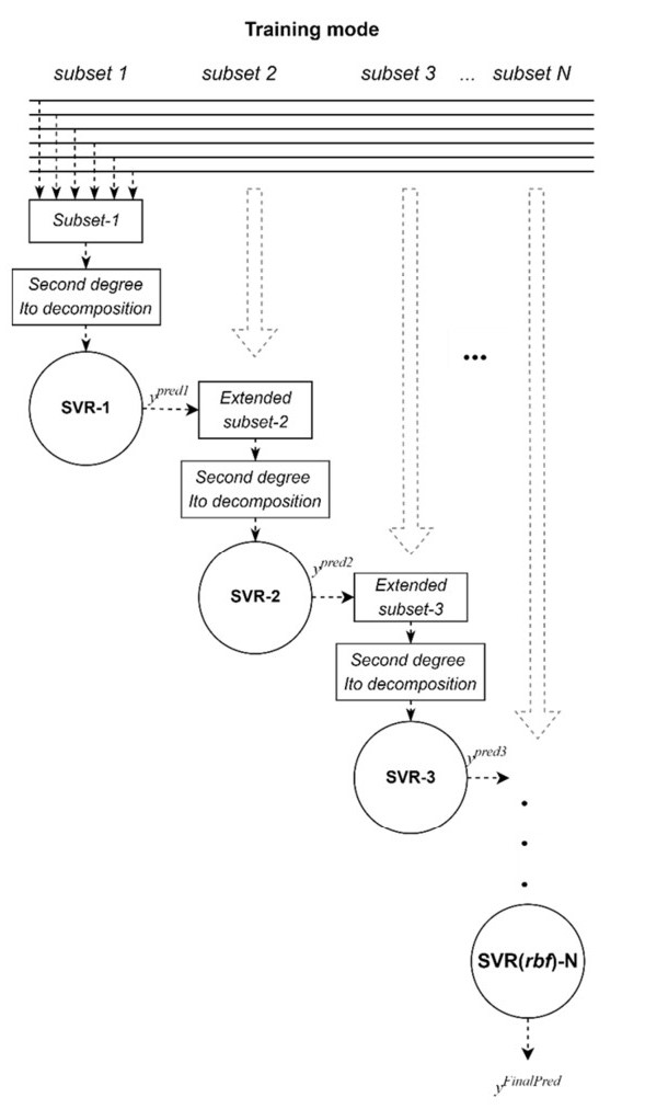
Biomedical data analysis is essential in current diagnosis, treatment, and patient condition monitoring. The large volumes of data that characterize this area require simple but accurate and fast methods of intellectual analysis to improve the level of medical services. Existing machine learning (ML) methods require many resources (time, memory, energy) when processing large datasets. Or they demonstrate a level of accuracy that is insufficient for solving a specific application task. In this paper, we developed a new ensemble model of increased accuracy for solving approximation problems of large biomedical data sets. The model is based on cascading of the ML methods and response surface linearization principles. In addition, we used Ito decomposition as a means of nonlinearly expanding the inputs at each level of the model. As weak learners, Support Vector Regression (SVR) with linear kernel was used due to many significant advantages demonstrated by this method among the existing ones. The training and application procedures of the developed SVR-based cascade model are described, and a flow chart of its implementation is presented. The modeling was carried out on a real-world tabular set of biomedical data of a large volume. The task of predicting the heart rate of individuals was solved, which provides the possibility of determining the level of human stress, and is an essential indicator in various applied fields. The optimal parameters of the SVR-based cascade model operating were selected experimentally. The authors shown that the developed model provides more than 20 times higher accuracy (according to Mean Squared Error (MSE)), as well as a significant reduction in the duration of the training procedure compared to the existing method, which provided the highest accuracy of work among those considered.
Citation: Ivan Izonin, Roman Tkachenko, Olexander Gurbych, Michal Kovac, Leszek Rutkowski, Rostyslav Holoven. A non-linear SVR-based cascade model for improving prediction accuracy of biomedical data analysis[J]. Mathematical Biosciences and Engineering, 2023, 20(7): 13398-13414. doi: 10.3934/mbe.2023597
Biomedical data analysis is essential in current diagnosis, treatment, and patient condition monitoring. The large volumes of data that characterize this area require simple but accurate and fast methods of intellectual analysis to improve the level of medical services. Existing machine learning (ML) methods require many resources (time, memory, energy) when processing large datasets. Or they demonstrate a level of accuracy that is insufficient for solving a specific application task. In this paper, we developed a new ensemble model of increased accuracy for solving approximation problems of large biomedical data sets. The model is based on cascading of the ML methods and response surface linearization principles. In addition, we used Ito decomposition as a means of nonlinearly expanding the inputs at each level of the model. As weak learners, Support Vector Regression (SVR) with linear kernel was used due to many significant advantages demonstrated by this method among the existing ones. The training and application procedures of the developed SVR-based cascade model are described, and a flow chart of its implementation is presented. The modeling was carried out on a real-world tabular set of biomedical data of a large volume. The task of predicting the heart rate of individuals was solved, which provides the possibility of determining the level of human stress, and is an essential indicator in various applied fields. The optimal parameters of the SVR-based cascade model operating were selected experimentally. The authors shown that the developed model provides more than 20 times higher accuracy (according to Mean Squared Error (MSE)), as well as a significant reduction in the duration of the training procedure compared to the existing method, which provided the highest accuracy of work among those considered.

| [1] |
N. Melnykova, N. Shakhovska, M. G. ml, V. Melnykov, Using big data for formalization the patient's personalized data, Proc. Comput. Sci., 155 (2019), 624–629. https://doi.org/10.1016/j.procs.2019.08.088 doi: 10.1016/j.procs.2019.08.088

|
| [2] |
K. Kakhi, R. Alizadehsani, H. M. D. Kabir, A. Khosravi, S. Nahavandi, U. R. Acharya, The internet of medical things and artificial intelligence: trends, challenges, and opportunities, Biocybern. Biomed. Eng., 42 (2022), 749–771. https://doi.org/10.1016/j.bbe.2022.05.008 doi: 10.1016/j.bbe.2022.05.008
|
| [3] |
I. H. Sarker, Machine learning: Algorithms, real-world applications and research directions, SN Comput. Sci., 2 (2021). https://doi.org/10.1007/s42979-021-00592-x doi: 10.1007/s42979-021-00592-x
|
| [4] |
I. Izonin, A. Trostianchyn, Z. Duriagina, R. Tkachenko, T. Tepla, N. Lotoshynska, The combined use of the wiener polynomial and SVM for material classification task in medical implants production, Int. J. Intell. Syst. Appl., 10 (2018), 40–47. https://doi.org/10.5815/ijisa.2018.09.05 doi: 10.5815/ijisa.2018.09.05
|
| [5] | I. Krak, O. Barmak, E. Manziuk, A. Kulias, Data classification based on the features reduction and piecewise linear separation, in International Conference on Intelligent Computing & Optimization, (2020), 282–289. https://doi.org/10.1007/978-3-030-33585-4_28 |
| [6] | G. Heitz, S. Gould, A. Saxena, D. Koller, Cascaded Classification Models: Combining Models for Holistic Scene Understanding, 2008. Available from: https://proceedings.neurips.cc/paper/2008/hash/072b030ba126b2f4b2374f342be9ed44-Abstract.html |
| [7] |
S. Kim, H. Park, W. Jung, K. Lim, Predicting heart rate variability parameters in healthy korean adults: A preliminary study, Inquiry, 58 (2021). https://doi.org/10.1177/00469580211056201 doi: 10.1177/00469580211056201
|
| [8] |
E. E. Tripoliti, T. G. Papadopoulos, G. S. Karanasiou, K. K. Naka, D. I. Fotiadis, Heart failure: Diagnosis, severity estimation and prediction of adverse events through machine learning techniques, Comput. Struct. Biotechnol. J., 15 (2017), 26–47. https://doi.org/10.1016/j.csbj.2016.11.001 doi: 10.1016/j.csbj.2016.11.001
|
| [9] | L. Fang, X. Liu, X. Su, J. Ye, S. Dobson, P. Hui, et al., Bayesian inference federated learning for heart rate prediction, in International Conference on Wireless Mobile Communication and Healthcare, 362 (2021), 116–130. https://doi.org/10.1007/978-3-030-70569-5_8 |
| [10] |
M. Oyeleye, T. Chen, S. Titarenko, G. Antoniou, A predictive analysis of heart rates using machine learning techniques, Int. J. Environ. Res. Public Health, 19 (2022), 2417. https://doi.org/10.3390/ijerph19042417 doi: 10.3390/ijerph19042417
|
| [11] |
T. R. Mahesh, V. D. Kumar, V. V. Kumar, J. Asghar, O. Geman, G. Arulkumaran, et al., Adaboost ensemble methods using k-fold cross validation for survivability with the early detection of heart disease, Comput. Intell. Neurosci., 2022 (2022), 9005278. https://doi.org/10.1155/2022/9005278 doi: 10.1155/2022/9005278
|
| [12] |
P. Theerthagiri, Predictive analysis of cardiovascular disease using gradient boosting based learning and recursive feature elimination technique, Intell. Syst. Appl., 16 (2022), 200121. https://doi.org/10.1016/j.iswa.2022.200121 doi: 10.1016/j.iswa.2022.200121
|
| [13] |
S. Manimurugan, S. Almutairi, M. M. Aborokbah, C. Narmatha, S. Ganesan, N. Chilamkurti, et al., Two-stage classification model for the prediction of heart disease using iomt and artificial intelligence, Sensors, 22 (2022), 476. https://doi.org/10.3390/s22020476 doi: 10.3390/s22020476
|
| [14] |
R. Tkachenko, I. Izonin, I. Dronyuk, M. Logoyda, P. Tkachenko, Recovery of missing sensor data with grnn-based cascade scheme, Int. J. Sens. Wireless Commun. Control, 11 (2021), 531–541. https://doi.org/10.2174/2210327910999200813151904 doi: 10.2174/2210327910999200813151904
|
| [15] |
I. Izonin, R. Tkachenko, R. Holoven, M. Shavarskyi, S. Bukin, I. Shevchuk, Multistage SVR-RBF-based model for heart rate prediction of individuals, in International Conference of Artificial Intelligence, Medical Engineering, Education, 159 (2023), 211–220. https://doi.org/10.1007/978-3-031-24468-1_19 doi: 10.1007/978-3-031-24468-1_19
|
| [16] |
J. Hsia, C. Lin, Parameter selection for linear Support Vector Regression, IEEE Trans. Neural Networks Learn. Syst., 31 (2020), 5639–5644. https://doi.org/10.1109/TNNLS.2020.2967637 doi: 10.1109/TNNLS.2020.2967637
|
| [17] |
I. Izonin, R. Tkachenko, An approach towards the response surface linearization via ANN-based cascade scheme for regression modeling in Healthcare, Proc. Comput. Sci., 198 (2022), 724–729. https://doi.org/10.1016/j.procs.2021.12.313 doi: 10.1016/j.procs.2021.12.313
|
| [18] |
A. G. Ivakhnenko, Polynomial theory of complex systems, IEEE Trans. Syst. Man Cybern., 4 (1971), 364–378. https://doi.org/10.1109/TSMC.1971.4308320 doi: 10.1109/TSMC.1971.4308320
|
| [19] | V. Kotsovsky, A. Batyuk, On-line relaxation versus off-line spectral algorithm in the learning of polynomial neural units, in International Conference on Data Stream Mining and Processing, (2020), 3–21. https://doi.org/10.1007/978-3-030-61656-4_1 |
| [20] | Y. B. Youssef, M. Afif, R. Ksantini, S. Tabbane, A novel QoE model based on boosting Support Vector Regression, in 2018 IEEE Wireless Communications and Networking Conference (WCNC), (2018), 1–6. https://doi.org/10.1109/WCNC.2018.8377092 |
| [21] | V. Shanawad, Heart Rate Prediction to Monitor Stress Level, 2023. Available from: https://www.kaggle.com/datasets/vinayakshanawad/heart-rate-prediction-to-monitor-stress-level |
| [22] |
L. Mochurad, Y. Hladun, Modeling of psychomotor reactions of a person based on modification of the tapping test, Int. J. Comput., 20 (2021), 1–10. https://doi.org/10.47839/ijc.20.2.2166 doi: 10.47839/ijc.20.2.2166
|
| [23] | G. Shanmugasundaram, S. Yazhini, E. Hemapratha, S. Nithya, A comprehensive review on stress detection techniques, in 2019 IEEE International Conference on System, Computation, Automation and Networking (ICSCAN), (2019), 1–6. https://doi.org/10.1109/ICSCAN.2019.8878795 |
| [24] |
Y. S. Can, N. Chalabianloo, D. Ekiz, J. Fernandez-Alvarez, G. Riva, C. Ersoy, Personal stress-level clustering and decision-level smoothing to enhance the performance of ambulatory stress detection with smartwatches, IEEE Access, 8 (2020), 38146–38163. https://doi.org/10.1109/ACCESS.2020.2975351 doi: 10.1109/ACCESS.2020.2975351
|
| [25] | A. Hasanbasic, M. Spahic, D. Bosnjic, H. H. adzic, V. Mesic, O. Jahic, Recognition of stress levels among students with wearable sensors, in 2019 18th International Symposium INFOTEH-JAHORINA (INFOTEH), (2019), 1–4. https://doi.org/10.1109/INFOTEH.2019.8717754 |
| [26] | I. Izonin, B. Ilchyshyn, R. Tkachenko, M. Greguš, N. Shakhovska, C. Strauss, Towards data normalization task for the efficient mining of medical data, in 2022 12th International Conference on Advanced Computer Information Technologies (ACIT), (2022), 1–5. https://doi.org/10.1109/ACIT54803.2022.9913112 |
| [27] |
V. Shymanskyi, Y. Sokolovskyy, Finite element calculation of the linear elasticity problem for biomaterials with fractal structure, Open Bioinf. J., 14 (2021), 114–122. https://doi.org/10.2174/18750362021140100114 doi: 10.2174/18750362021140100114
|
| [28] | N. García-Pedrajas, D. Ortiz-Boyer, R. del Castillo-Gomariz, C. Hervás-Martínez, Cascade ensembles, in International Work-Conference on Artificial Neural Networks, (2005), 598–603. https://doi.org/10.1007/11494669_73 |
| [29] |
Y. V. Bodyanskiy, O. K. Tyshchenko, A hybrid cascade neural network with ensembles of extended neo-fuzzy neurons and its deep learning, in Conference on Information Technology, Systems Research and Computational Physics, 945 (2018), 164–174. https://doi.org/10.1007/978-3-030-18058-4_13 doi: 10.1007/978-3-030-18058-4_13
|
| [30] |
A. G. Ivakhnenko, Development of models of optimal complexity using self-organization theory, Int. J. Comput. Inf. Sci., 8 (1979), 111–127. https://doi.org/10.1007/BF00989666 doi: 10.1007/BF00989666
|
| [31] |
J. Zhou, Y. Ye, J. Jiang, Kernel principal components based cascade forest towards disease identification with human microbiota, BMC Med. Inform. Decis. Mak., 21 (2021), 360. https://doi.org/10.1186/s12911-021-01705-5 doi: 10.1186/s12911-021-01705-5
|
| [32] | I. Tsmots, O. Skorokhoda, Methods and VLSI-structures for neural element implementation, in 2010 Proceedings of VIth International Conference on Perspective Technologies and Methods in MEMS Design, (2010), 135–135. |
| [33] |
I. G. Kryvonos, I.V. Krak, O. V. Barmak, A. S. Ternov, V. O. Kuznetsov, Information technology for the analysis of mimic expressions of human emotional states, Cybern. Syst. Anal., 51 (2015), 25–33. https://doi.org/10.1007/s10559-015-9693-1 doi: 10.1007/s10559-015-9693-1
|
| [34] |
V. Babenko, A. Panchyshyn, L. Zomchak, M. Nehrey, Z. Artym-Drohomyretska, T. Lahotskyi, Classical machine learning methods in economics research: Macro and micro level examples, WSEAS Trans. Bus. Econ., 18 (2021), 209–217. https://doi.org/10.37394/23207.2021.18.22 doi: 10.37394/23207.2021.18.22
|
| [35] | D. Chumachenko, T. Chumachenko, I. Meniailov, P. Pyrohov, I. Kuzin, R. Rodyna, On-line data processing, simulation and forecasting of the coronavirus disease (COVID-19) propagation in ukraine based on machine learning approach, in International Conference on Data Stream Mining and Processing, 1158 (2020), 372–382. https://doi.org/10.1007/978-3-030-61656-4_25 |
Figures(3) / Tables(3)

Ivan Izonin, Roman Tkachenko, Olexander Gurbych, Michal Kovac, Leszek Rutkowski, Rostyslav Holoven. A non-linear SVR-based cascade model for improving prediction accuracy of biomedical data analysis[J]. Mathematical Biosciences and Engineering, 2023, 20(7): 13398-13414. doi: 10.3934/mbe.2023597


 DownLoad: