The origin, location and cause of Parkinson's oscillation are not clear at present. In this paper, we establish a new cortex-basal ganglia model to study the origin mechanism of Parkinson beta oscillation. Unlike many previous models, this model includes two direct inhibitory projections from the globus pallidus external (GPe) segment to the cortex. We first obtain the critical calculation formula of Parkinson's oscillation by using the method of Quasilinear analysis. Different from previous studies, the formula obtained in this paper can include the self-feedback connection of GPe. Then, we use the bifurcation analysis method to systematically explain the influence of some key parameters on the oscillation. We find that the bifurcation principle of different cortical nuclei is different. In general, the increase of the discharge capacity of the nuclei will cause oscillation. In some special cases, the sharp reduction of the discharge rate of the nuclei will also cause oscillation. The direction of bifurcation simulation is consistent with the critical condition curve. Finally, we discuss the characteristics of oscillation amplitude. At the beginning of the oscillation, the amplitude is relatively small; with the evolution of oscillation, the amplitude will gradually strengthen. This is consistent with the experimental phenomenon. In most cases, the amplitude of cortical inhibitory nuclei (CIN) is greater than that of cortical excitatory nuclei (CEX), and the two direct inhibitory projections feedback from GPe can significantly reduce the amplitude gap between them. We calculate the main frequency of the oscillation generated in this model, which basically falls between 13 and 30 Hz, belonging to the typical beta frequency band oscillation. Some new results obtained in this paper can help to better understand the origin mechanism of Parkinson's disease and have guiding significance for the development of experiments.
Citation: Minbo Xu, Bing Hu, Weiting Zhou, Zhizhi Wang, Luyao Zhu, Jiahui Lin, Dingjiang Wang. The mechanism of Parkinson oscillation in the cortex: Possible evidence in a feedback model projecting from the globus pallidus to the cortex[J]. Mathematical Biosciences and Engineering, 2023, 20(4): 6517-6550. doi: 10.3934/mbe.2023281
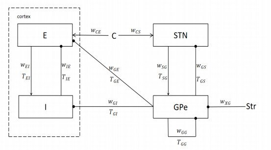
The origin, location and cause of Parkinson's oscillation are not clear at present. In this paper, we establish a new cortex-basal ganglia model to study the origin mechanism of Parkinson beta oscillation. Unlike many previous models, this model includes two direct inhibitory projections from the globus pallidus external (GPe) segment to the cortex. We first obtain the critical calculation formula of Parkinson's oscillation by using the method of Quasilinear analysis. Different from previous studies, the formula obtained in this paper can include the self-feedback connection of GPe. Then, we use the bifurcation analysis method to systematically explain the influence of some key parameters on the oscillation. We find that the bifurcation principle of different cortical nuclei is different. In general, the increase of the discharge capacity of the nuclei will cause oscillation. In some special cases, the sharp reduction of the discharge rate of the nuclei will also cause oscillation. The direction of bifurcation simulation is consistent with the critical condition curve. Finally, we discuss the characteristics of oscillation amplitude. At the beginning of the oscillation, the amplitude is relatively small; with the evolution of oscillation, the amplitude will gradually strengthen. This is consistent with the experimental phenomenon. In most cases, the amplitude of cortical inhibitory nuclei (CIN) is greater than that of cortical excitatory nuclei (CEX), and the two direct inhibitory projections feedback from GPe can significantly reduce the amplitude gap between them. We calculate the main frequency of the oscillation generated in this model, which basically falls between 13 and 30 Hz, belonging to the typical beta frequency band oscillation. Some new results obtained in this paper can help to better understand the origin mechanism of Parkinson's disease and have guiding significance for the development of experiments.

| [1] |
E. Wressle, C. Engstrand, A. K. Granérus, Living with Parkinson's disease: elderly patients' and relatives' perspective on daily living, Aust. Occup. Ther. J., 54 (2007), 131–139. https://doi.org/10.1111/j.1440-1630.2006.00610.x doi: 10.1111/j.1440-1630.2006.00610.x

|
| [2] |
P. Mahlknecht, A. Gasperi, P. Willeit, S. Kiechl, H. Stockner, J. Willeit, et al., Prodromal Parkinson's disease as defined per MDS research criteria in the general elderly community, Mov. Disord., 31 (2016), 1405–1408. https://doi.org/10.1002/mds.26674 doi: 10.1002/mds.26674
|
| [3] |
M. Politis, K. Wu, S. Molloy, P. G. Bain, K. R. Chaudhuri, P. Piccini, Parkinson's disease symptoms: the patient's perspective, Mov. Disord., 25 (2010), 1646–1651. https://doi.org/10.1002/mds.23135 doi: 10.1002/mds.23135
|
| [4] |
C. Váradi, Clinical features of Parkinson's disease: the evolution of critical symptoms, Biology, 9 (2020), 103. https://doi.org/10.3390/biology9050103 doi: 10.3390/biology9050103
|
| [5] |
D. J. Surmeier, Determinants of dopaminergic neuron loss in Parkinson's disease, FEBS J., 285 (2018), 3657–3668. https://doi.org/10.1111/febs.14607 doi: 10.1111/febs.14607
|
| [6] |
C. Raza, R. Anjum, Parkinson's disease: Mechanisms, translational models and management strategies, Life Sci., 226 (2019), 77–90. https://doi.org/10.1016/j.lfs.2019.03.057 doi: 10.1016/j.lfs.2019.03.057
|
| [7] |
A. B. Holt, E. Kormann, A. Gulberti, M. Pötter-Nerger, C. G. McNamara, H. Cagnan, et al., Phase-dependent suppression of beta oscillations in Parkinson's disease patients, J. Neurosci., 39 (2019), 1119–1134. https://doi.org/10.1523/JNEUROSCI.1913-18.2018 doi: 10.1523/JNEUROSCI.1913-18.2018
|
| [8] |
A. Singh, R. C. Cole, A. I. Espinoza, D. Brown, J. F. Cavanagh, N. S. Narayanana, Frontal theta and beta oscillations during lower-limb movement in Parkinson's disease, Clin. Neurophysiol., 131 (2020), 694-702. https://doi.org/10.1016/j.clinph.2019.12.399 doi: 10.1016/j.clinph.2019.12.399
|
| [9] |
M. H. Trager, M. M. Koop, A. Velisar, Z. Blumenfeld, J. S. Nikolau, E. J. Quinn, et al., Subthalamic beta oscillations are attenuated after withdrawal of chronic high frequency neurostimulation in Parkinson's disease, Neurobiol. Dis., 96 (2016), 22–30. https://doi.org/10.1016/j.nbd.2016.08.003 doi: 10.1016/j.nbd.2016.08.003
|
| [10] |
C. Hammond, H. Bergman, P. Brown, Pathological synchronization in Parkinson's disease: networks, models and treatments, Trends Neurosci., 30 (2007), 357–364. https://doi.org/10.1016/j.tins.2007.05.004 doi: 10.1016/j.tins.2007.05.004
|
| [11] |
Z. Wang, B. Hu, W. Zhou, M. Xu, D. Wang, Hopf bifurcation mechanism analysis in an improved cortex-basal ganglia network with distributed delays: An application to Parkinson's disease, Chaos, Solitons Fractals, 166 (2023), 113022. https://doi.org/10.1016/j.chaos.2022.113022 doi: 10.1016/j.chaos.2022.113022
|
| [12] |
B. Hu, X. Diao, H. Guo, et al., The beta oscillation conditions in a simplified basal ganglia network, Cogn Neurodynamics, 13(2019), 201-217. https://doi.org/10.1007/s11571-018-9514-0 doi: 10.1007/s11571-018-9514-0
|
| [13] |
A. B. Holt, T. I. Netoff, Origins and suppression of oscillations in a computational model of Parkinson's disease, J. Comput. Neurosci., 37 (2014), 505–521. https://doi.org/10.1007/s10827-014-0523-7 doi: 10.1007/s10827-014-0523-7
|
| [14] |
A. B. Holt, E. Kormann, A. Gulberti, M. Pötter-Nerger, C. G. McNamara, H. Cagnan, et al., Phase-dependent suppression of beta oscillations in Parkinson's disease patients, J. Neurosci., 39 (2019), 1119–1134. https://doi.org/10.1523/JNEUROSCI.1913-18.2018 doi: 10.1523/JNEUROSCI.1913-18.2018
|
| [15] |
L. L. Grado, M. D. Johnson, T. I. Netoff, Bayesian adaptive dual control of deep brain stimulation in a computational model of Parkinson's disease, PLoS Comput. Biol., 14 (2018), e1006606. https://doi.org/10.1371/journal.pcbi.1006606 doi: 10.1371/journal.pcbi.1006606
|
| [16] |
J. E. Fleming, E. Dunn, M. M. Lowery, Simulation of closed-loop deep brain stimulation control schemes for suppression of pathological beta oscillations in Parkinson's disease, Front. Neurosci., 14 (2020), 166. https://doi.org/10.3389/fnins.2020.00166 doi: 10.3389/fnins.2020.00166
|
| [17] |
A. B. Holt, D. Wilson, M. Shinn, J. Moehlis, T. I. Netoff, Phasic burst stimulation: a closed-loop approach to tuning deep brain stimulation parameters for Parkinson's disease, PLoS Comput. Biol., 12 (2016), e1005011. https://doi.org/10.1371/journal.pcbi.1005011 doi: 10.1371/journal.pcbi.1005011
|
| [18] |
K. Kumaravelu, D. T. Brocker, W. M. Grill, A biophysical model of the cortex-basal ganglia-thalamus network in the 6-OHDA lesioned rat model of Parkinson's disease, J. Comput. Neurosci., 40 (2016), 207–229. https://doi.org/10.1007/s10827-016-0593-9 doi: 10.1007/s10827-016-0593-9
|
| [19] |
A. J. N. Holgado, J. R. Terry, R. Bogacz, Conditions for the generation of beta oscillations in the subthalamic nucleus-globus pallidus network, J. Neurosci., 30 (2010), 12340–12352. https://doi.org/10.1523/JNEUROSCI.0817-10.2010 doi: 10.1523/JNEUROSCI.0817-10.2010
|
| [20] |
A. Pavlides, S. J. Hogan, R. Bogacz, Improved conditions for the generation of beta oscillations in the subthalamic nucleus-globus pallidus network, Eur. J. Neurosci., 36 (2012), 2229–2239. https://doi.org/10.1111/j.1460-9568.2012.08105.x doi: 10.1111/j.1460-9568.2012.08105.x
|
| [21] |
Gillies, D. Willshaw, Z. Li, Subthalamic-pallidal interactions are critical in determining normal and abnormal functioning of the basal ganglia, Proc. R. Soc. London, Ser. B, 269 (2002), 545–551. https://doi.org/10.1098/rspb.2001.1817 doi: 10.1098/rspb.2001.1817
|
| [22] |
J. E. Rubin, D. Terman, High frequency stimulation of the subthalamic nucleus eliminates pathological thalamic rhythmicity in a computational model, J. Comput. Neurosci., 16 (2004), 211–235. https://doi.org/10.1023/B:JCNS.0000025686.47117.67 doi: 10.1023/B:JCNS.0000025686.47117.67
|
| [23] |
D. Terman, J. E. Rubin, A. C. Yew, C. J. Wilson, Activity patterns in a model for the subthalamopallidal network of the basal ganglia, J. Neurosci., 22 (2002), 2963–2976. https://doi.org/10.1523/JNEUROSCI.22-07-02963.2002 doi: 10.1523/JNEUROSCI.22-07-02963.2002
|
| [24] |
B. Hu, M. Xu, L. Zhu, J. Lin, Z. Wang, D. Wang, et al., A bidirectional Hopf bifurcation analysis of Parkinson's oscillation in a simplified basal ganglia model, J. Theor. Biol., 536 (2022), 110979. https://doi.org/10.1016/j.jtbi.2021.110979 doi: 10.1016/j.jtbi.2021.110979
|
| [25] |
S. R. Cole, R. van der Meij, E. J. Peterson, C. de Hemptinne, P. A. Starr, B. Voytek, Nonsinusoidal beta oscillations reflect cortical pathophysiology in Parkinson's disease, J. Neurosci., 37 (2017), 4830–4840. https://doi.org/10.1523/JNEUROSCI.2208-16.2017 doi: 10.1523/JNEUROSCI.2208-16.2017
|
| [26] |
B. Pollok, V. Krause, W. Martsch, C. Wach, A. Schnitzler, M. Südmeyer, Motor‐cortical oscillations in early stages of Parkinson's disease, J.Physiol., 590 (2012), 3203–3212. https://doi.org/10.1113/jphysiol.2012.231316 doi: 10.1113/jphysiol.2012.231316
|
| [27] |
S. J. van Albada, P. A. Robinson, Mean-field modeling of the basal ganglia-thalamocortical system. I: Firing rates in healthy and parkinsonian states, J. Theor. Biol., 257 (2009), 642–663. https://doi.org/10.1016/j.jtbi.2008.12.018 doi: 10.1016/j.jtbi.2008.12.018
|
| [28] |
S. J. van Albada, R. T. Gray, P. M. Drysdale, P. A. Robinson, Mean-field modeling of the basal ganglia-thalamocortical system. Ⅱ: dynamics of parkinsonian oscillations, J. Theor. Biol., 257 (2009), 664–688. https://doi.org/10.1016/j.jtbi.2008.12.013 doi: 10.1016/j.jtbi.2008.12.013
|
| [29] |
G. W. Arbuthnott, M. Garcia-Munoz, Are the symptoms of parkinsonism cortical in origin?, Comput. Struct. Biotechnol. J., 15 (2017), 21–25. https://doi.org/10.1016/j.csbj.2016.10.006 doi: 10.1016/j.csbj.2016.10.006
|
| [30] |
C. F. Underwood, L. C. Parr-Brownlie, Primary motor cortex in Parkinson's disease: Functional changes and opportunities for neurostimulation, Neurobiol. Dis., 147 (2021), 105159. https://doi.org/10.1016/j.nbd.2020.105159 doi: 10.1016/j.nbd.2020.105159
|
| [31] |
M. D. Bevan, P. J. Magill, D. Terman, J. P. Bolam, C. J Wilson, Move to the rhythm: oscillations in the subthalamic nucleus-external globus pallidus network, Trends Neurosci., 25 (2002), 525–531. https://doi.org/10.1016/S0166-2236(02)02235-X doi: 10.1016/S0166-2236(02)02235-X
|
| [32] |
A. Pavlides, S. J. Hogan, R. Bogacz, Computational models describing possible mechanisms for generation of excessive beta oscillations in Parkinson's disease, PLoS Comput. Biol., 11 (2015), e1004609. https://doi.org/10.1371/journal.pcbi.1004609 doi: 10.1371/journal.pcbi.1004609
|
| [33] |
Y. Chen, J. Wang, Y. Kang, M. B. Ghori, Emergence of beta oscillations of a resonance model for Parkinson's disease, Neural Plast., 2020 (2020), 1–15. https://doi.org/10.1155/2020/8824760 doi: 10.1155/2020/8824760
|
| [34] |
M. M. McGregor, A. B. Nelson, Circuit mechanisms of Parkinson's disease, Neuron, 101 (2019), 1042–1056. https://doi.org/10.1016/j.neuron.2019.03.004 doi: 10.1016/j.neuron.2019.03.004
|
| [35] |
M. D. Humphries, J. A. Obeso, J. K. Dreyer, Insights into Parkinson's disease from computational models of the basal ganglia, J. Neurol., Neurosurg. Psychiatry, 89 (2018), 1181–1188. https://doi.org/10.1136/jnnp-2017-315922 doi: 10.1136/jnnp-2017-315922
|
| [36] |
B. C. M. van Wijk, H. Cagnan, V. Litvak, V. Litvak, A. A. Kühn, K. J. Friston, et al., Generic dynamic causal modelling: An illustrative application to Parkinson's disease, NeuroImage, 181 (2018), 818–830. https://doi.org/10.1016/j.neuroimage.2018.08.039 doi: 10.1016/j.neuroimage.2018.08.039
|
| [37] |
M. C. Chen, L. Ferrari, M. D. Sacchet, L. C. Foland-Ross, M. Qiu, I. H. Gotlib, et al., Identification of a direct GABA ergic pallidocortical pathway in rodents, Eur. J. Neurosci., 41 (2015), 748–759. https://doi.org/10.1111/ejn.12822 doi: 10.1111/ejn.12822
|
| [38] |
A. Saunders, I. A. Oldenburg, V. K. Berezovskii, C. A. Johnson, N. D. Kingery, H. L. Elliott, et al., A direct GABAergic output from the basal ganglia to frontal cortex, Nature, 521 (2015), 85–89. https://doi.org/10.1038/nature14179 doi: 10.1038/nature14179
|
| [39] | P. R. Castillo, E. H. Middlebrooks, S. S. Grewal, L. Okromelidze, J. F. Meschia, A. Quinones-Hinojosa, et al., Globus pallidus externus deep brain stimulation treats insomnia in a patient with Parkinson disease, in Mayo Clinic Proceedings, Elsevier, 95 (2020), 419–422. https://doi.org/10.1016/j.mayocp.2019.11.020 |
| [40] |
J. Dong, S. Hawes, J. Wu, W. Le, H. Cai, Connectivity and functionality of the globus pallidus externa under normal conditions and Parkinson's disease, Front. Neural Circuits, 15 (2021), 8. https://doi.org/10.3389/fncir.2021.645287 doi: 10.3389/fncir.2021.645287
|
| [41] |
T. Tsuboi, M. Charbel, D. T. Peterside, M. Rana, A. Elkouzi, W. Deeb, et al., Pallidal connectivity profiling of stimulation-induced dyskinesia in Parkinson's disease, Mov. Disord., 36 (2021), 380–388. https://doi.org/10.1002/mds.28324 doi: 10.1002/mds.28324
|
| [42] |
R. G. Burciu, D. E. Vaillancourt, Imaging of motor cortex physiology in Parkinson's disease, Mov. Disord., 33 (2018), 1688–1699. https://doi.org/10.1002/mds.102 doi: 10.1002/mds.102
|
| [43] |
G. Foffani, J. A. Obeso, A cortical pathogenic theory of Parkinson's disease, Neuron, 99 (2018), 1116–1128. https://doi.org/10.1016/j.neuron.2018.07.028 doi: 10.1016/j.neuron.2018.07.028
|
| [44] |
A. Guerra, D. Colella, M. Giangrosso, A. Cannavacciuolo, G. Paparella, G. Fabbrini, et al., Driving motor cortex oscillations modulates bradykinesia in Parkinson's disease, Brain, 145 (2022), 224–236. https://doi.org/10.1093/brain/awab257 doi: 10.1093/brain/awab257
|
| [45] |
Z. Wang, B. Hu, L. Zhu, J, Lin, M. Xu, D. Wang, Hopf bifurcation analysis for Parkinson oscillation with heterogeneous delays: A theoretical derivation and simulation analysis, Commun. Nonlinear. Sci., 114 (2022), 106614. https://doi.org/10.1016/j.cnsns.2022.106614 doi: 10.1016/j.cnsns.2022.106614
|
| [46] |
T. P. Vogels, K. Rajan, L. F. Abbott, Neural network dynamics, Annu. Rev. Neurosci., 28 (2005), 357–376. https://doi.org/10.1146/annurev.neuro.28.061604.135637 doi: 10.1146/annurev.neuro.28.061604.135637
|
| [47] |
H. Kita, Y. Tachibana, A. Nambu, S. Chiken, Balance of monosynaptic excitatory and disynaptic inhibitory responses of the globus pallidus induced after stimulation of the subthalamic nucleus in the monkey, J. Neurosci., 25 (2005), 8611–8619. https://doi.org/10.1523/JNEUROSCI.1719-05.2005 doi: 10.1523/JNEUROSCI.1719-05.2005
|
| [48] |
J. T. Paz, J. M. Deniau, S. Charpier, Rhythmic bursting in the cortico-subthalamo-pallidal network during spontaneous genetically determined spike and wave discharges, J. Neurosci., 25 (2005), 2092–2101. https://doi.org/10.1523/JNEUROSCI.4689-04.2005 doi: 10.1523/JNEUROSCI.4689-04.2005
|
| [49] |
H. Kita, S. T. Kitai, Intracellular study of rat globus pallidus neurons: membrane properties and responses to neostriatal, subthalamic and nigral stimulation, Brain Res., 564 (1991), 296–305. https://doi.org/10.1016/0006-8993(91)91466-E doi: 10.1016/0006-8993(91)91466-E
|
| [50] |
M. A. Lebedev, S. P. Wise, Oscillations in the premotor cortex: single-unit activity from awake, behaving monkeys, Exp. Brain Res., 130 (2000), 195–215. https://doi.org/10.1007/s002210050022 doi: 10.1007/s002210050022
|
| [51] |
W. Schultz, R. Romo, Neuronal activity in the monkey striatum during the initiation of movements, Exp. Brain Res., 71 (1988), 431–436. https://doi.org/10.1007/BF00247503 doi: 10.1007/BF00247503
|
| [52] |
N. E. Hallworth, C. J. Wilson, M. D. Bevan, Apamin-sensitive small conductance calcium-activated potassium channels, through their selective coupling to voltage-gated calcium channels, are critical determinants of the precision, pace, and pattern of action potential generation in rat subthalamic nucleus neurons in vitro, J. Neurosci., 23 (2003), 7525–7542. https://doi.org/10.1523/JNEUROSCI.23-20-07525.2003 doi: 10.1523/JNEUROSCI.23-20-07525.2003
|
| [53] |
H. Kita, Globus pallidus external segment, Prog. Brain Res., 160 (2007), 111–133. https://doi.org/10.1016/S0079-6123(06)60007-1 doi: 10.1016/S0079-6123(06)60007-1
|
| [54] |
H. Kita, A. Nambu, K. Kaneda, Y. Tachibana, M. Takada, Role of ionotropic glutamatergic and GABAergic inputs on the firing activity of neurons in the external pallidum in awake monkeys, J. Neurophysiol., 92 (2004), 3069–3084. https://doi.org/10.1152/jn.00346.2004 doi: 10.1152/jn.00346.2004
|
| [55] |
H. Nakanishi, H. Kita, S. T. Kitai, Intracellular study of rat substantia nigra pars reticulata neurons in an in vitro slice preparation: electrical membrane properties and response characteristics to subthalamic stimulation, Brain Res., 437 (1987), 45–55. https://doi.org/10.1016/0006-8993(87)91525-3 doi: 10.1016/0006-8993(87)91525-3
|
| [56] |
K. Fujimoto, H. Kita, Response characteristics of subthalamic neurons to the stimulation of the sensorimotor cortex in the rat, Brain Res., 609 (1993), 185–192. https://doi.org/10.1016/0006-8993(93)90872-K doi: 10.1016/0006-8993(93)90872-K
|
| [57] |
A. Gillies, D. Willshaw, Membrane channel interactions underlying rat subthalamic projection neuron rhythmic and bursting activity, J. Neurophysiol., 95 (2006), 2352–2365. https://doi.org/10.1152/jn.00525.2005 doi: 10.1152/jn.00525.2005
|
| [58] |
H. Kita, S. T. Kitai, Intracellular study of rat globus pallidus neurons: membrane properties and responses to neostriatal, subthalamic and nigral stimulation, Brain Res., 564 (1991), 296–305. https://doi.org/10.1016/0006-8993(91)91466-E doi: 10.1016/0006-8993(91)91466-E
|
| [59] |
Y. Hirai, M. Morishima, F. Karube, Y. Kawaguchi, Specialized cortical subnetworks differentially connect frontal cortex to parahippocampal areas, J. Neurosci., 32 (2012), 1898–1913. https://doi.org/10.1523/JNEUROSCI.2810-11.2012 doi: 10.1523/JNEUROSCI.2810-11.2012
|
| [60] |
Y. H. Tanaka, Y. Tanaka, F. Fujiyama, T. Furuta, Y. Yanagawa, T. Kaneko, Local connections of layer 5 GABAergic interneurons to corticospinal neurons, Front. Neural Circuits, 5 (2011), 12. https://doi.org/10.3389/fncir.2011.00012 doi: 10.3389/fncir.2011.00012
|
| [61] |
M. H. Higgs, S. J. Slee, W. J. Spain, Diversity of gain modulation by noise in neocortical neurons: regulation by the slow afterhyperpolarization conductance, J. Neurosci., 26 (2006), 8787–8799. https://doi.org/10.1523/JNEUROSCI.1792-06.2006 doi: 10.1523/JNEUROSCI.1792-06.2006
|
| [62] |
A. L. Barth, J. F. A. Poulet, Experimental evidence for sparse firing in the neocortex, Trends Neurosci., 35 (2012), 345–355. https://doi.org/10.1016/j.tins.2012.03.008 doi: 10.1016/j.tins.2012.03.008
|
| [63] |
A. P. Prudnikov, Y. A. Brychkov, O. I. Marichev, Integrals and series: direct laplace transforms, Routledge, 2018. https://doi.org/10.1201/9780203750643 doi: 10.1201/9780203750643
|
| [64] |
K. Udupa, N. Bahl, Z. Ni, C. Gunraj, F. Mazzella, E. Moro, et al., Cortical plasticity induction by pairing subthalamic nucleus deep-brain stimulation and primary motor cortical transcranial magnetic stimulation in Parkinson's disease, J. Neurosci., 36 (2016), 396–404. https://doi.org/10.1523/JNEUROSCI.2499-15.2016 doi: 10.1523/JNEUROSCI.2499-15.2016
|
| [65] |
M. Dagan, T. Herman, R. Harrison, J. Zhou, N. Giladi, G. Ruffini, et al., Multitarget transcranial direct current stimulation for freezing of gait in Parkinson's disease, Mov. Disord., 33 (2018), 642–646. https://doi.org/10.1002/mds.27300 doi: 10.1002/mds.27300
|
| [66] |
E. Lattari, S. S. Costa, C. Campos, A. J. Oliveira, S. Machado, G. A. M. Neto, Can transcranial direct current stimulation on the dorsolateral prefrontal cortex improves balance and functional mobility in Parkinson's disease?, Neurosci. Lett., 636 (2017), 165–169. https://doi.org/10.1016/j.neulet.2016.11.019 doi: 10.1016/j.neulet.2016.11.019
|


Figures(22) / Tables(2)

Minbo Xu, Bing Hu, Weiting Zhou, Zhizhi Wang, Luyao Zhu, Jiahui Lin, Dingjiang Wang. The mechanism of Parkinson oscillation in the cortex: Possible evidence in a feedback model projecting from the globus pallidus to the cortex[J]. Mathematical Biosciences and Engineering, 2023, 20(4): 6517-6550. doi: 10.3934/mbe.2023281


 DownLoad: