The Covid illness (COVID-19), which has emerged, is a highly infectious viral disease. This disease led to thousands of infected cases worldwide. Several mathematical compartmental models have been examined recently in order to better understand the Covid disease. The majority of these models rely on integer-order derivatives, which are incapable of capturing the fading memory and crossover behaviour observed in many biological phenomena. Similarly, the Covid disease is investigated in this paper by exploring the elements of COVID-19 pathogens using the non-integer Atangana-Baleanu-Caputo derivative. Using fixed point theory, we demonstrate the existence and uniqueness of the model's solution. All basic properties for the given model are investigated in addition to Ulam-Hyers stability analysis. The numerical scheme is based on Lagrange's interpolation polynomial developed to estimate the model's approximate solution. Using real-world data, we simulate the outcomes for different fractional orders in Matlab to illustrate the transmission patterns of the present Coronavirus-19 epidemic through graphs.
Citation: Ihtisham Ul Haq, Nigar Ali, Shabir Ahmad. A fractional mathematical model for COVID-19 outbreak transmission dynamics with the impact of isolation and social distancing[J]. Mathematical Modelling and Control, 2022, 2(4): 228-242. doi: 10.3934/mmc.2022022
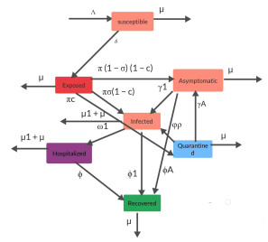
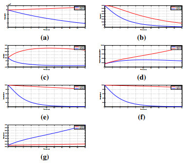
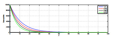
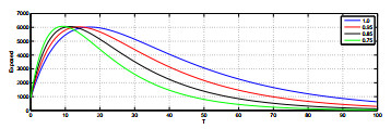
The Covid illness (COVID-19), which has emerged, is a highly infectious viral disease. This disease led to thousands of infected cases worldwide. Several mathematical compartmental models have been examined recently in order to better understand the Covid disease. The majority of these models rely on integer-order derivatives, which are incapable of capturing the fading memory and crossover behaviour observed in many biological phenomena. Similarly, the Covid disease is investigated in this paper by exploring the elements of COVID-19 pathogens using the non-integer Atangana-Baleanu-Caputo derivative. Using fixed point theory, we demonstrate the existence and uniqueness of the model's solution. All basic properties for the given model are investigated in addition to Ulam-Hyers stability analysis. The numerical scheme is based on Lagrange's interpolation polynomial developed to estimate the model's approximate solution. Using real-world data, we simulate the outcomes for different fractional orders in Matlab to illustrate the transmission patterns of the present Coronavirus-19 epidemic through graphs.

| [1] | J. Li, Y. Wang, S. Gilmour, M. Wang, D. Yoneoka, Y. Wang, et al., Estimation of the epidemic properties of the 2019 novel coronavirus: A mathematical modeling study, J. Am. Math. Soc., (2020). |
| [2] |
Q. Lin, S. Zhao, D. Gao, Y. Lou, S. Yang, S. S. Musa, et al., A conceptual model for the coronavirus disease 2019 (COVID-19) outbreak in Wuhan, China with individual reaction and governmental action, Int. J. Infect. Dis., 93 (2020), 211–216. https://doi.org/10.1016/j.ijid.2020.02.058 doi: 10.1016/j.ijid.2020.02.058

|
| [3] | World Health Organization and others, Coronavirus disease 2019 (COVID-19): situation report, 51 World Health Organization, (2020). |
| [4] | J. Li, Y. Wang, S. Gilmour, M. Wang, D. Yoneoka, Y. Wang, et al., Interim guidance for homeless service providers to plan and respond to coronavirus disease 2019 (COVID-19), J. Am. Math. Soc., (2020), 1–10. |
| [5] |
A. J. Kucharski, T. W. Russell, C. Diamond, Y. Liu, J. Edmunds, S. Funk, et al., Early dynamics of transmission and control of COVID-19: a mathematical modelling study, The lancet infectious diseases, 20 (2020), 553–558. https://doi.org/10.1016/S1473-3099(20)30144-4 doi: 10.1016/S1473-3099(20)30144-4
|
| [6] | Y. Liu, A. A. Gayle, A. Wilder-Smith, J. Rocklov, The reproductive number of COVID-19 is higher compared to SARS coronavirus, J. Travel Med., (2020). |
| [7] | S. Zhao, H. Chen, Modeling the epidemic dynamics and control of COVID-19 outbreak in China, Quant. Biol., 1 (2020), 1–9. |
| [8] | H. Song, F. Liu, F. Li, X. Cao, H. Wang, Z. Jia, et al., The impact of isolation on the transmission of COVID-19 and estimation of potential second epidemic in China, Preprints, (2020). |
| [9] |
S. A. Sarkodie, P. A. Owusu, Global assessment of environment, health and economic impact of the novel coronavirus (COVID-19), Environment, Development and Sustainability, 23 (2021), 5005–5015. https://doi.org/10.1007/s10668-020-00801-2 doi: 10.1007/s10668-020-00801-2
|
| [10] |
I. U. Haq, N. Ali, S. Ahmad, T. Akram, A Hybrid Interpolation Method for Fractional PDEs and Its Applications to Fractional Diffusion and Buckmaster Equations, Math. Probl. Eng., 2022 (2022). https://doi.org/10.1155/2022/2517602 doi: 10.1155/2022/2517602
|
| [11] |
Y. Chen, D. Guo, Molecular mechanisms of coronavirus RNA capping and methylation, Virol. Sin., 31 (2016), 3–11. https://doi.org/10.1007/s12250-016-3726-4 doi: 10.1007/s12250-016-3726-4
|
| [12] | I. U. Haq, N. Ali, K. S. Nisar, An optimal control strategy and Grünwald-Letnikov finite-difference numerical scheme for the fractional-order COVID-19 model, Mathematical Modelling and Numerical Simulation with Applications, 2 (2022), 108–116. |
| [13] |
H. Lu, C. W. Stratton, Y.-W. Tang, Outbreak of pneumonia of unknown etiology in Wuhan, China: the mystery and the miracle, J. Med. Virol., 92 (2020), 401–402. https://doi.org/10.1002/jmv.25678 doi: 10.1002/jmv.25678
|
| [14] |
E. Rinott, I. Youngster, Y. E. Lewis, Reduction in COVID-19 patients requiring mechanical ventilation following implementation of a national COVID-19 vaccination program—Israel, December 2020–February 2021, Morbidity and Mortality Weekly Report, 70 (2021), 326. https://doi.org/10.15585/mmwr.mm7009e3 doi: 10.15585/mmwr.mm7009e3
|
| [15] |
P. Ingrid Johnston, Australia's public health response to COVID-19: what have we done, and where to from here? Aust. NZ J. Publ. Heal., 44 (2020), 440. https://doi.org/10.1111/1753-6405.13051 doi: 10.1111/1753-6405.13051
|
| [16] | S. Zhao, H. Chen, Modeling the epidemic dynamics and control of COVID-19 outbreak in China, Quant. Biol., 2 (2020), 1–9. |
| [17] | H. Song, F. Liu, F. Li, X. Cao, H. Wang, Z. Jia, et al., The impact of isolation on the transmission of COVID-19 and estimation of potential second epidemic in China, Preprints, (2020). |
| [18] |
J. Li, Y. Wang, S. Gilmour, M. Wang, D. Yoneoka, Y. Wang, et al., A new study on two different vaccinated fractional-order COVID-19 models via numerical algorithms, J. King Saud Univ. Sci., 34 (2022), 101914. https://doi.org/10.1016/j.jksus.2022.101914 doi: 10.1016/j.jksus.2022.101914
|
| [19] |
J. Li, Y. Wang, S. Gilmour, M. Wang, D. Yoneoka, Y. Wang, et al., Projections and fractional dynamics of COVID-19 with optimal control strategies, Chaos, Solitons & Fractals, 145 (2022), 110689. https://doi.org/10.1016/j.chaos.2021.110689 doi: 10.1016/j.chaos.2021.110689
|
| [20] |
K. N. Nabi, H. Abboubakar, P. Kumar, Forecasting of COVID-19 pandemic: From integer derivatives to fractional derivatives, Chaos, Solitons & Fractals, 141 (2020), 110283. https://doi.org/10.1016/j.chaos.2020.110283 doi: 10.1016/j.chaos.2020.110283
|
| [21] |
N. P. Jewell, J. A. Lewnard, B. L. Jewell, Predictive mathematical models of the COVID-19 pandemic: underlying principles and value of projections, Jama, 323 (2020), 1893–1894. https://doi.org/10.1001/jama.2020.6585 doi: 10.1001/jama.2020.6585
|
| [22] |
M. S. Khan, M. Ozair, T. Hussain, J. Gomez-Aguilar, Bifurcation analysis of a discrete-time compartmental model for hypertensive or diabetic patients exposed to COVID-19, The European Physical Journal Plus, 136 (2021), 1–26. https://doi.org/10.1140/epjp/s13360-021-01862-6 doi: 10.1140/epjp/s13360-021-01862-6
|
| [23] |
R. P. Yadav, R. Verma, A numerical simulation of fractional order mathematical modeling of COVID-19 disease in case of Wuhan China, Chaos, Solitons & Fractals, 140 (2020), 110124. https://doi.org/10.1016/j.chaos.2020.110124 doi: 10.1016/j.chaos.2020.110124
|
| [24] |
P. Pandey, Y.-M. Chu, J. Gomez-Aguilar, H. Jahanshahi, A. A. Aly, A novel fractional mathematical model of COVID-19 epidemic considering quarantine and latent time, Results Phys., 26 (2021), 104286. https://doi.org/10.1016/j.rinp.2021.104286 doi: 10.1016/j.rinp.2021.104286
|
| [25] |
A. Khan, H. M. Alshehri, T. Abdeljawad, Q. M. Al-Mdallal, H. Khan, Stability analysis of fractional nabla difference COVID-19 model, Results Phys., 122 (2021), 103888. https://doi.org/10.1016/j.rinp.2021.103888 doi: 10.1016/j.rinp.2021.103888
|
| [26] |
M. S. Abdo, K. Shah, H. A. Wahash, S. K. Panchal, On a comprehensive model of the novel coronavirus (COVID-19) under Mittag-Leffler derivative, Chaos, Solitons and Fractals, 135 (2020), 109867. https://doi.org/10.1016/j.chaos.2020.109867 doi: 10.1016/j.chaos.2020.109867
|
| [27] |
P. Pandey, J. Gomez-Aguilar, M. K. Kaabar, Z. Siri, A. M. Abd Allah, Mathematical modeling of COVID-19 pandemic in India using Caputo-Fabrizio fractional derivative, Comput. Biol. Med., 145 (2022), 105518. https://doi.org/10.1016/j.compbiomed.2022.105518 doi: 10.1016/j.compbiomed.2022.105518
|
| [28] |
M. Al-Refai, T. Abdeljawad, Analysis of the fractional diffusion equations with fractional derivative of non-singular kernel, Advances in Difference Equations, 2017 (2017), 1–12. https://doi.org/10.1186/s13662-017-1356-2 doi: 10.1186/s13662-017-1356-2
|
| [29] |
S. Hasan, A. El-Ajou, S. Hadid, M. Al-Smadi, S. Momani, Atangana-Baleanu fractional framework of reproducing kernel technique in solving fractional population dynamics system, Chaos, Solitons & Fractals, 133 (2020), 109624. https://doi.org/10.1016/j.chaos.2020.109624 doi: 10.1016/j.chaos.2020.109624
|
| [30] |
S. A. Khan, K. Shah, G. Zaman, F. Jarad, Existence theory and numerical solutions to smoking model under Caputo-Fabrizio fractional derivative, Chaos: An Interdisciplinary Journal of Nonlinear Science, 29 (2019), 013128. https://doi.org/10.1063/1.5079644 doi: 10.1063/1.5079644
|
| [31] |
M. L. Morgado, N. J. Ford, P. M. Lima, Analysis and numerical methods for fractional differential equations with delay, J. Comput. Appl. Math., 252 (2020), 159–168. https://doi.org/10.1016/j.cam.2012.06.034 doi: 10.1016/j.cam.2012.06.034
|
| [32] |
R. Garrappa, Trapezoidal methods for fractional differential equations: Theoretical and computational aspects, Math. Comput. Simulat., 110 (22015), 96–112. https://doi.org/10.1016/j.matcom.2013.09.012 doi: 10.1016/j.matcom.2013.09.012
|
| [33] |
K. Shah, Z. A. Khan, A. Ali, R. Amin, H. Khan, A. Khan, Haar wavelet collocation approach for the solution of fractional order COVID-19 model using Caputo derivative, Alex. Eng. J., 59 (2020), 3221–3231. https://doi.org/10.1016/j.aej.2020.08.028 doi: 10.1016/j.aej.2020.08.028
|
| [34] |
A. Atangana, J. Gomez-Aguilar, Numerical approximation of Riemann-Liouville definition of fractional derivative: from Riemann-Liouville to Atangana-Baleanu, Numerical Methods for Partial Differential Equations, 34 (2018), 1502–1523. https://doi.org/10.1002/num.22195 doi: 10.1002/num.22195
|
| [35] |
R. Resmawan, L. Yahya, Sensitivity analysis of mathematical model of coronavirus disease (COVID-19) transmission, Cauchy, 6 (2020), 91–99. https://doi.org/10.18860/ca.v6i2.9165 doi: 10.18860/ca.v6i2.9165
|
| [36] |
A. S. Shaikh, I. N. Shaikh, K. S. Nisar, A mathematical model of COVID-19 using fractional derivative: outbreak in India with dynamics of transmission and control, Advances in Difference Equations, 2020 (2020), 1–19. https://doi.org/10.1186/s13662-020-02834-3 doi: 10.1186/s13662-020-02834-3
|
| [37] |
B. Tang, X. Wang, Q. Li, N. L. Bragazzi, S. Tang, Y. Xiao, et al., Estimation of the transmission risk of the 2019-nCoV and its implication for public health interventions, J. Clin. Med., 9 (2020), 462. https://doi.org/10.3390/jcm9020462 doi: 10.3390/jcm9020462
|
| [38] |
C. N. Ngonghala, E. Iboi, S. Eikenberry, M. Scotch, C. R. MacIntyre, M. H. Bonds, et al., Mathematical assessment of the impact of non-pharmaceutical interventions on curtailing the 2019 novel Coronavirus, Math. Biosci., 135 (2020), 108364. https://doi.org/10.1016/j.mbs.2020.108364 doi: 10.1016/j.mbs.2020.108364
|
| [39] |
I. ul Haq, Analytical Approximate Solution Of Non-Linear Problem By Homotopy Perturbation Method (Hpm), Matrix Science Mathematic, 3 (2029), 20–24. https://doi.org/10.26480/msmk.01.2019.20.24 doi: 10.26480/msmk.01.2019.20.24
|
| [40] |
J. Solıs-Perez, J. Gomez-Aguilar, A. Atangana, X. You, J. Gu, C. Hao, et al., Novel numerical method for solving variable-order fractional differential equations with power, exponential and Mittag-Leffler laws, Chaos, Solitons & Fractals, 114 (2018), 175–185. https://doi.org/10.1016/j.chaos.2018.06.032 doi: 10.1016/j.chaos.2018.06.032
|
| [41] |
J. Solıs-Perez, J. Gomez-Aguilar, A. Atangana, Novel numerical method for solving variable-order fractional differential equations with power, exponential and Mittag-Leffler laws, Chaos, Solitons & Fractals, 114 (2018), 175–185. https://doi.org/10.1016/j.chaos.2018.06.032 doi: 10.1016/j.chaos.2018.06.032
|
| [42] |
C. Li, A. Chen, Numerical methods for fractional partial differential equations, International Journal of Computer Mathematics, 95 (2018), 1048–1099. https://doi.org/10.1080/00207160.2017.1343941 doi: 10.1080/00207160.2017.1343941
|
| [43] | J. Wang, K. Shah, A. Ali, Existence and Hyers-Ulam stability of fractional nonlinear impulsive switched coupled evolution equations, Math. Method. Appl. Sci., 41 (2018), 2392–2402. |
| [44] |
M. Ahmad, A. Zada, J. Alzabut, Hyers–Ulam stability of a coupled system of fractional differential equations of Hilfer–Hadamard type, Demonstratio Mathematica, 52 (2019), 283–295. https://doi.org/10.1515/dema-2019-0024 doi: 10.1515/dema-2019-0024
|
| [45] |
A. Khan, H. Khan, J. Gomez-Aguilar, T. Abdeljawad, Existence and Hyers-Ulam stability for a nonlinear singular fractional differential equations with Mittag-Leffler kernel, Chaos, Solitons & Fractals, 127 (2019), 422–427. https://doi.org/10.1016/j.chaos.2019.07.026 doi: 10.1016/j.chaos.2019.07.026
|
| [46] |
V. S. Panwar, P. S. Uduman, J. G omez-Aguilar, Mathematical modeling of coronavirus disease COVID-19 dynamics using CF and ABC non-singular fractional derivatives, Chaos, Solitons & Fractals, 145 (2021), 110757. https://doi.org/10.1016/j.chaos.2021.110757 doi: 10.1016/j.chaos.2021.110757
|
| [47] |
M. Ahmad, A. Zada, J. Alzabut, Hyers–Ulam stability of a coupled system of fractional differential equations of Hilfer–Hadamard type, Demonstratio Mathematica, 52 (2019), 283–295. https://doi.org/10.1515/dema-2019-0024 doi: 10.1515/dema-2019-0024
|
Figures(10) / Tables(2)
Ihtisham Ul Haq, Nigar Ali, Shabir Ahmad. A fractional mathematical model for COVID-19 outbreak transmission dynamics with the impact of isolation and social distancing[J]. Mathematical Modelling and Control, 2022, 2(4): 228-242. doi: 10.3934/mmc.2022022


 DownLoad: