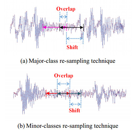
As an indispensable part of large Computer Numerical Control machine tool, rolling bearing faults diagnosis is particularly important. However, due to the imbalanced distribution and partially missing of collected monitoring data, such diagnostic issue generally emerging in manufacturing industry is still hardly to be solved. Thus, a multilevel recovery diagnosis model for rolling bearing faults from imbalanced and partially missing monitoring data is formulated in this paper. Firstly, a regulable resampling plan is designed to handle the imbalanced distribution of data. Secondly, a multilevel recovery scheme is formed to deal with partially missing. Thirdly, an improved sparse autoencoder based multilevel recovery diagnosis model is built to identify the health status of rolling bearings. Finally, the diagnostic performance of the designed model is verified by artificial faults and practical faults tests, respectively.
Citation: Jing Yang, Guo Xie, Yanxi Yang, Qijun Li, Cheng Yang. A multilevel recovery diagnosis model for rolling bearing faults from imbalanced and partially missing monitoring data[J]. Mathematical Biosciences and Engineering, 2023, 20(3): 5223-5242. doi: 10.3934/mbe.2023242
As an indispensable part of large Computer Numerical Control machine tool, rolling bearing faults diagnosis is particularly important. However, due to the imbalanced distribution and partially missing of collected monitoring data, such diagnostic issue generally emerging in manufacturing industry is still hardly to be solved. Thus, a multilevel recovery diagnosis model for rolling bearing faults from imbalanced and partially missing monitoring data is formulated in this paper. Firstly, a regulable resampling plan is designed to handle the imbalanced distribution of data. Secondly, a multilevel recovery scheme is formed to deal with partially missing. Thirdly, an improved sparse autoencoder based multilevel recovery diagnosis model is built to identify the health status of rolling bearings. Finally, the diagnostic performance of the designed model is verified by artificial faults and practical faults tests, respectively.

| [1] |
P. Yang, Z. Li, Y. Yu, J. Shi, M. Sun, Studies on fault diagnosis of dissolved oxygen sensor based on GA-SVM, Math. Biosci. Eng., 18 (2021), 386–399. https://doi.org/10.3934/mbe.2021021 doi: 10.3934/mbe.2021021

|
| [2] |
J. Yang, G. Xie, Y. Yang, X. Li, L. Mu, S. Takahashi, H. Mochizuki, An improved deep network for intelligent diagnosis of machinery faults with similar features, IEEJ, 14 (2019), 1851–1864. https://doi.org/10.1002/tee.23012 doi: 10.1002/tee.23012
|
| [3] |
G. Xie, J. Yang, Y. Yang, An improved sparse autoencoder and multi-level denoising strategy for diagnosing early multiple intermittent faults, IEEE Trans. Syst. Man Cybern.: Syst., 52 (2022), 869–880. https://doi.org/10.1109/TSMC.2020.3005433 doi: 10.1109/TSMC.2020.3005433
|
| [4] |
Y. Zhou, A. Kumar, C. Parkash, G. Vashishtha, H. Tang, J. Xiang, A novel entropy-based sparsity measure for prognosis of bearing defects and development of a sparsogram to select sensitive filtering band of an axial piston pump, Measurement, 203 (2022), 111997. https://doi.org/10.1016/j.measurement.2022.111997 doi: 10.1016/j.measurement.2022.111997
|
| [5] |
N. Xu, G. Zhang, L. Yang, Z. Shen, M. Xu, L. Chang, Research on thermoeconomic fault diagnosis for marine low speed two stroke diesel engine, Math. Biosci. Eng., 19 (2022), 5393–5408. https://doi.org/10.3934/mbe.2022253 doi: 10.3934/mbe.2022253
|
| [6] |
J. Yang, G. Xie, Y. Yang, A key-factor denoising strategy for quasi periodic non-stationary incipient faults diagnosis, Measurement, 197 (2022), 111304. https://doi.org/10.1016/j.measurement.2022.111304 doi: 10.1016/j.measurement.2022.111304
|
| [7] |
J. Yang, G. Xie, Y. Yang, Y. Zhang, W. Liu, Deep model integrated with data correlation analysis for multiple intermittent faults diagnosis, ISA Trans., 95 (2019), 306–319. https://doi.org/10.1016/j.isatra.2019.05.021 doi: 10.1016/j.isatra.2019.05.021
|
| [8] |
J. Yang, Y. Yang, G. Xie, Diagnosis of incipient fault based on sliding-scale resampling strategy and improved deep autoencoder, IEEE Sens. J., 20 (2020), 8336–8348. https://doi.org/10.1109/JSEN.2020.2976523 doi: 10.1109/JSEN.2020.2976523
|
| [9] |
Y. Wang, D. Zhao, Y. Li, S. X. Ding, Unbiased minimum variance fault and state estimation for linear discrete time-varying two-dimensional systems, IEEE Trans. Autom. Control, 62 (2017), 5463–5469. https://doi.org/10.1109/TAC.2017.2697210 doi: 10.1109/TAC.2017.2697210
|
| [10] |
R. Sun, Y. Han, Y. Wang, Design of generalized fault diagnosis observer and active adaptive fault tolerant controller for aircraft control system, Math. Biosci. Eng., 19 (2022), 5591–5609. https://doi.org/10.3934/mbe.2022262 doi: 10.3934/mbe.2022262
|
| [11] |
R. Zhao, R. Yan, Z. Chen, K. Mao, P. Wang, R. X. Gao, Deep learning and its applications to machine health monitoring, Mech. Syst. Signal Process., 115 (2019), 213–237. https://doi.org/10.1016/j.ymssp.2018.05.050 doi: 10.1016/j.ymssp.2018.05.050
|
| [12] |
W. Li, X. Zhong, H. Shao, B. Cai, X. Yang, Multi-mode data augmentation and fault diagnosis of rotating machinery using modified ACGAN designed with new framework, Adv. Eng. Inf., 52 (2022), 101552. https://doi.org/10.1016/j.aei.2022.101552 doi: 10.1016/j.aei.2022.101552
|
| [13] |
X. Chen, G. Cheng, H. Li, M. Zhang, Diagnosing planetary gear faults using the fuzzy entropy of LMD and ANFIS, J. Mech. Sci. Technol., 30 (2016), 2453–2462. https://doi.org/10.1007/s12206-016-0505-y doi: 10.1007/s12206-016-0505-y
|
| [14] |
M. R. Praveen, M. Saimurugan, Health monitoring of a gear box using vibration signal analysis, Appl. Mech. Mater., 813–814 (2015), 1012–1017. https://doi.org/10.4028/www.scientific.net/AMM.813-814.1012 doi: 10.4028/www.scientific.net/AMM.813-814.1012
|
| [15] |
A. E. Prosvirin, M. Islam, J. Kim, J. Kim, Rub-impact fault diagnosis using an effective IMF selection technique in ensemble empirical mode decomposition and hybrid feature models, Sensors, 18 (2018), 2040. https://doi.org/10.3390/s18072040 doi: 10.3390/s18072040
|
| [16] |
Y. Wang, G. Xu, L. Liang, K. Jiang, Detection of weak transient signals based on wavelet packet transform and manifold learning for rolling element bearing fault diagnosis, Mech. Syst. Signal Process., 54–55 (2015), 259–276. https://doi.org/10.1016/j.ymssp.2014.09.002 doi: 10.1016/j.ymssp.2014.09.002
|
| [17] |
Y. LeCun, Y. Bengio, G. Hinton, Deep learning, Nature, 521 (2015), 436–444. https://doi.org/10.1038/nature14539 doi: 10.1038/nature14539
|
| [18] |
Y. Zhou, G. Zhi, W. Chen, Q. Qian, D. He, B. Sun, et. al., A new tool wear condition monitoring method based on deep learning under small samples, Measurement, 189 (2022), 110622. https://doi.org/10.1016/j.measurement.2021.110622 doi: 10.1016/j.measurement.2021.110622
|
| [19] |
S. Jia, Z. Yu, A. Onken, Y. Tian, T. Huang, J. K. Liu, Neural system identification with spike-triggered non-negative matrix factorization, IEEE Trans. Cybern., 52 (2022), 4772–4783. https://doi.org/10.1109/TCYB.2020.3042513 doi: 10.1109/TCYB.2020.3042513
|
| [20] |
J. Yang, Y. Bai, G. Li, M. Liu, X. Liu, A novel method of diagnosing premature ventricular contraction based on sparse auto-encoder and softmax regression, Bio.-Med. Mater. Eng., 26 (2015), 1549–1558. https://doi.org/10.3233/BME-151454 doi: 10.3233/BME-151454
|
| [21] | J. Deng, Z. Zhang, E. Marchi, B. Schuller, Sparse autoencoder-based feature transfer learning for speech emotion recognition, in 2013 Humaine Association Conference on Affective Computing and Intelligent Interaction, (2013), 511–516. https://doi.org/10.1109/ACⅡ.2013.90 |
| [22] |
J. Yang, G. Xie, Yanxi Yang, An improved ensemble fusion autoencoder model for fault diagnosis from imbalanced and incomplete data, Control Eng. Pract., 98 (2020), 104358. https://doi.org/10.1016/j.conengprac.2020.104358 doi: 10.1016/j.conengprac.2020.104358
|
| [23] |
R. Liu, B. Yang, E. Zio, X. Chen, Artificial intelligence for fault diagnosis of rotating machinery: A review, Mech. Syst. Signal Process., 108 (2018), 33–47. https://doi.org/10.1016/j.ymssp.2018.02.016 doi: 10.1016/j.ymssp.2018.02.016
|
| [24] |
C. Lu, Z. Wang, W. Qin, J. Ma, Fault diagnosis of rotary machinery components using a stacked denoising autoencoder-based health state identification, Signal Process., 130 (2017), 377–388. https://doi.org/10.1016/j.sigpro.2016.07.028 doi: 10.1016/j.sigpro.2016.07.028
|
| [25] |
M. Sohaib, C. Kim, J. Kim, A hybrid feature model and deep-learning-based bearing fault diagnosis, Sensors, 17 (2017), 2876–2891. https://doi.org/10.3390/s17122876 doi: 10.3390/s17122876
|
| [26] |
J. Sun, C. Yan, J. Wen, Intelligent bearing fault diagnosis method combining compressed data acquisition and deep learning, IEEE Trans. Instrum. Meas., 67 (2018), 185–195. https://doi.org/10.1109/TIM.2017.2759418 doi: 10.1109/TIM.2017.2759418
|
| [27] |
G. Liu, H. Bao, B. Han, A stacked autoencoder-based deep neural network for achieving gearbox fault diagnosis, Math. Probl. Eng., 2018 (2018), 1–10. https://doi.org/10.1155/2018/5105709 doi: 10.1155/2018/5105709
|
| [28] |
Y. Qian, Y. Liang, M. Li, G. Feng, X. Shi, A resampling ensemble algorithm for classification of imbalance problems, Neurocomputing, 143 (2014), 57–67. https://doi.org/10.1016/j.neucom.2014.06.021 doi: 10.1016/j.neucom.2014.06.021
|
| [29] |
S. Cateni, V. Colla, M. Vannucci, A method for resampling imbalanced datasets in binary classification tasks for real-world problems, Neurocomputing, 135 (2014), 32–41. https://doi.org/10.1016/j.neucom.2013.05.059 doi: 10.1016/j.neucom.2013.05.059
|
| [30] |
X. Han, R. Cui, Y. Lan, Y. Kang, J. Deng, N. Jia, A Gaussian mixture model based combined resampling algorithm for classification of imbalanced credit data sets, Int. J. Mach. Learn. Cybern., 10 (2019), 3687–3699. https://doi.org/10.1007/s13042-019-00953-2 doi: 10.1007/s13042-019-00953-2
|
| [31] | K. Loparo, Case western reserve university bearing data center, 2013. Available from: http://csegroups.case.edu/bearingdatacenter/pages. |
| [32] |
Y. Qi, C. Shen, D. Wang, J. Shi, X. Jiang, Z. Zhu, Stacked sparse autoencoder-based deep network for fault diagnosis of rotating machinery, IEEE Access, 5 (2017), 15066–15079. https://doi.org/10.1109/ACCESS.2017.2728010 doi: 10.1109/ACCESS.2017.2728010
|
| [33] |
Z. Liu, X. Chen, Z. He, Z. Shen, LMD method and multi-class RWSVM of fault diagnosis for rotating machinery using condition monitoring information, Sensors, 13 (2013), 8679–8694. https://doi.org/10.3390/s130708679 doi: 10.3390/s130708679
|
| [34] |
F. Zhou, Y. Gao, C. Wen, A novel multimode fault classification method based on deep learning, J. Control Sci. Eng., 2017 (2017), 1–14. https://doi.org/10.1155/2017/3583610 doi: 10.1155/2017/3583610
|
| [35] | C. Lessmeier, J. K. Kimotho, D. Zimmer, W. Sextro, Condition monitoring of bearing damage in electromechanical drive systems by using motor current signals of electric motors: A benchmark data set for data-driven classification, in 2016 European Conference of the Prognostics and Health Management Society, (2016), 1–18. |


Figures(13) / Tables(8)

Jing Yang, Guo Xie, Yanxi Yang, Qijun Li, Cheng Yang. A multilevel recovery diagnosis model for rolling bearing faults from imbalanced and partially missing monitoring data[J]. Mathematical Biosciences and Engineering, 2023, 20(3): 5223-5242. doi: 10.3934/mbe.2023242


 DownLoad: