A class of explicit implicit alternating difference schemes for generalized time fractional Fisher equation

Xiao Qin; Xiaozhong Yang; Peng Lyu; Xiao Qin; Xiaozhong Yang; Peng Lyu

doi:10.3934/math.2021663

AIMS Mathematics

2021, Volume 6, Issue 10: 11449-11466. doi: 10.3934/math.2021663

Previous Article Next Article

Research article Special Issues

A class of explicit implicit alternating difference schemes for generalized time fractional Fisher equation

School of Mathematics and Physics, North China Electric Power University, Beijing 102206, China

Received: 31 May 2021 Accepted: 04 August 2021 Published: 09 August 2021
MSC : 65M06, 65M12

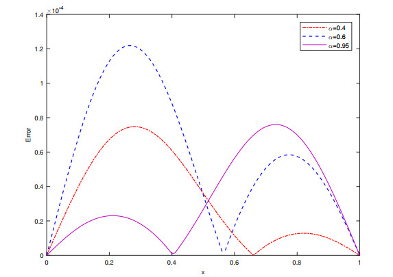
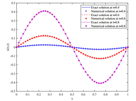
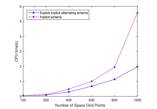
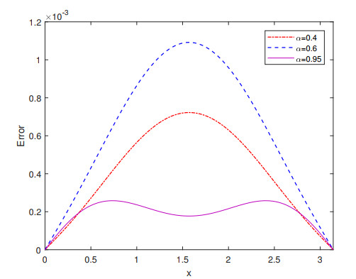
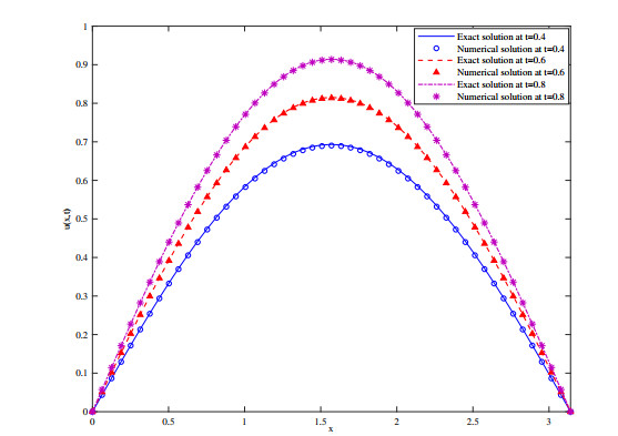
The generalized time fractional Fisher equation is one of the significant models to describe the dynamics of the system. The study of effective numerical techniques for the equation has important scientific significance and application value. Based on the alternating technique, this article combines the classical explicit difference scheme and the implicit difference scheme to construct a class of explicit implicit alternating difference schemes for the generalized time fractional Fisher equation. The unconditional stability and convergence with order $ O\left({\tau }^{2-\alpha }+{h}^{2}\right) $ of the proposed schemes are analyzed. Numerical examples are performed to verify the theoretical analysis. Compared with the classical implicit difference scheme, the calculation cost of the explicit implicit alternating difference schemes is reduced by almost $ 60 $%. Numerical experiments show that the explicit implicit alternating difference schemes are also suitable for solving the time fractional Fisher equation with initial weak singularity and have an accuracy of order $ O\left({\tau }^{\alpha }+{h}^{2}\right) $, which verify that the methods proposed in this paper are efficient for solving the generalized time fractional Fisher equation.
- generalized time fractional Fisher equation,
- explicit implicit alternating difference scheme,
- stability,
- convergence,
- numerical experiments
Citation: Xiao Qin, Xiaozhong Yang, Peng Lyu. A class of explicit implicit alternating difference schemes for generalized time fractional Fisher equation[J]. AIMS Mathematics, 2021, 6(10): 11449-11466. doi: 10.3934/math.2021663

Related Papers:

Abstract

The generalized time fractional Fisher equation is one of the significant models to describe the dynamics of the system. The study of effective numerical techniques for the equation has important scientific significance and application value. Based on the alternating technique, this article combines the classical explicit difference scheme and the implicit difference scheme to construct a class of explicit implicit alternating difference schemes for the generalized time fractional Fisher equation. The unconditional stability and convergence with order $ O\left({\tau }^{2-\alpha }+{h}^{2}\right) $ of the proposed schemes are analyzed. Numerical examples are performed to verify the theoretical analysis. Compared with the classical implicit difference scheme, the calculation cost of the explicit implicit alternating difference schemes is reduced by almost $ 60 $%. Numerical experiments show that the explicit implicit alternating difference schemes are also suitable for solving the time fractional Fisher equation with initial weak singularity and have an accuracy of order $ O\left({\tau }^{\alpha }+{h}^{2}\right) $, which verify that the methods proposed in this paper are efficient for solving the generalized time fractional Fisher equation.

References

[1]	J. Sabatier, O. P. Agrawal, J. A. T. Machado, Advances in fractional calculus: theoretical developments and applications in physics and engineering, Beijing: Beijing World Publishing Corporation, 2014.
[2]	V. V. Uchaikin, Fractional derivatives for physicists and engineers: Volume II: applications, Beijing: Higher Education Press, 2013.
[3]	T. Sandev, Z. Tomovski, Fractional equations and models: theory and applications, Berlin: Springer, 2019.
[4]	K. Diethelm, The analysis of fractional differential equations, New York: Springer, 2010.
[5]	C. Ravichandran, J. J. Trujillo, Controllability of impulsive fractional functional integro-differential equations in Banach spaces, J. Funct. Spaces Appl., (2013), 812501.
[6]	M. A. Alqudah, C. Ravichandran, T. Abdeljawad, N. Valliammal, New results on Caputo fractional-order neutral differential inclusions without compactness, Adv. Differ. Equ., 2019 (2019), 528. doi: 10.1186/s13662-019-2455-z
[7]	M. Goyal, H. M. Baskonus, A. Prakash, An efficient technique for a time fractional model of lassa hemorrhagic fever spreading in pregnant women, Eur. Phys. J. Plus, 134 (2019), 482. doi: 10.1140/epjp/i2019-12854-0
[8]	A. Kumar, H. V. S. Chauhan, C. Ravichandran, K. S. Nisar, D. Baleanu, Existence of solutions of non-autonomous fractional differential equations with integral impulse condition, Adv. Differ. Equ., 2020 (2020), 434. doi: 10.1186/s13662-020-02888-3
[9]	D. F. Li, H. L. Liao, W. W. Sun, J. L. Wang, J. W. Zhang, Analysis of $L1$-Galerkin FEMs for time-fractional nonlinear parabolic problems, Commun. Comput. Phys., 24 (2018), 86–103.
[10]	A. Majeed, M. Kamran, M. K. Iqbal, D. Baleanu, Solving time fractional Burgers' and Fisher's equations using cubic B-spline approximation method, Adv. Differ. Equ., 2020 (2020), 175. doi: 10.1186/s13662-020-02619-8
[11]	J. Ross, A. F. Villaverde, J. R. Banga, S. Vazquez, F. Moran, A generalized Fisher equation and its utility in chemical kinetics, Proc. Natl. Acad. Sci. U. S. A., 107 (2010), 12777–12781. doi: 10.1073/pnas.1008257107
[12]	M. Merdan, Solutions of time-fractional reaction-diffusion equation with modified Riemann-Liouville derivative, Int. J. Phys. Sci., 7 (2012), 2317–2326.
[13]	T. Sardar, S. Rana, J. Chattopadhyay, A mathematical model of dengue transmission with memory, Commun. Nonlinear Sci. Numer. Simul., 22 (2015), 511–525. doi: 10.1016/j.cnsns.2014.08.009
[14]	B. L. Guo, X. K. Pu, F. H. Huang, Fractional partial differential equations and their numerical solutions, Beijing: Science Press, 2015.
[15]	F. W. Liu, P. H. Zhuang, Q. X. Liu, Numerical methods and their application of fractional partial differential equations, Beijing: Science Press, 2015 (in Chinese).
[16]	C. P. Li, M. Cai, Theory and numerical approximations of fractional integrals and derivatives, Philadelphia: SIAM, 2019.
[17]	S. S. Ray, The comparison of two reliable methods for the accurate solution of fractional Fisher type equation, Eng. Comput., 34 (2017), 2598–2613. doi: 10.1108/EC-03-2017-0074
[18]	M. M. Al Qurashi, Z. Korpinar, D. Baleanu, M. Inc, A new iterative algorithm on the time-fractional Fisher equation: residual power series method, Adv. Mech. Eng., 9 (2017), 1–8.
[19]	P. Veeresha, D. G. Prakasha, H. M. Baskonus, Novel simulations to the time-fractional Fisher's equation, Math. Sci., 13 (2019), 33–42. doi: 10.1007/s40096-019-0276-6
[20]	A. Secer, M. Cinar, A Jacobi wavelet collocation method for fractional Fisher's equation in time, Thermal Sci., 24 (2020), S119–S129. doi: 10.2298/TSCI20S1119S
[21]	A. Majeed, M. Kamran, M. Abbas, J. Singh, An efficient numerical technique for solving time-fractional generalized Fisher's equation, Front. Phys., 8 (2020), 293. doi: 10.3389/fphy.2020.00293
[22]	X. D. Zhang, Y. N. He, L. L. Wei, B. Tang, S. L. Wang, A fully discrete local discontinuous Galerkin method for one-dimensional time-fractional Fisher's equation, Int. J. Comput. Math., 91 (2014), 2021–2038. doi: 10.1080/00207160.2013.866233
[23]	M. Alquran, K. Al-Khaled, T. Sardar, J. Chattopadhyay, Revisited Fisher's equation in a new outlook: a fractional derivative approach, Phys. A, 438 (2015), 81–93. doi: 10.1016/j.physa.2015.06.036
[24]	A. Atangana, On the new fractional derivative and application to nonlinear Fisher's reaction-diffusion equation, Appl. Math. Comput., 273 (2016), 948–956.
[25]	S. B. Yuste, J. Quintana-Murillo, A finite difference method with non-uniform timesteps for fractional diffusion equations, Comput. Phys. Commun., 183 (2012), 2594–2600. doi: 10.1016/j.cpc.2012.07.011
[26]	E. Sousa, A second order explicit finite difference method for the fractional advection diffusion equation, Comput. Math. Appl., 64 (2012), 3141–3152. doi: 10.1016/j.camwa.2012.03.002
[27]	Y. N. Zhang, Z. Z. Sun, H. L. Liao, Finite difference methods for the time fractional diffusion equation on non-uniform meshes, J. Comput. Phys., 265 (2014), 195–210. doi: 10.1016/j.jcp.2014.02.008
[28]	F. Al-Shibani, A. Ismail, Compact Crank-Nicolson and Du Fort-Frankel method for the solution of the time fractional diffusion equation, Int. J. Comput. Methods, 12 (2015), 1550041. doi: 10.1142/S0219876215500413
[29]	H. L. Liao, Y. N. Zhang, Y. Zhao, H. S. Shi, Stability and convergence of modified Du Fort-Frankel schemes for solving time-fractional subdiffusion equations, J. Sci. Comput., 61 (2014), 629–648. doi: 10.1007/s10915-014-9841-1
[30]	Y. Liu, Y. W. Du, H. Li, S. He, W. Gao, Finite difference/finite element method for a nonlinear time-fractional fourth-order reaction-diffusion problem, Comput. Math. Appl., 70 (2015), 573–591. doi: 10.1016/j.camwa.2015.05.015
[31]	M. M. Khader, K. M. Saad, A numerical approach for solving the fractional Fisher equation using Chebyshev spectral collocation method, Chaos Solitons Fractals, 110 (2018), 169–177. doi: 10.1016/j.chaos.2018.03.018
[32]	J. X. Zhang, X. Z. Yang, A class of efficient difference method for time fractional reaction-diffusion equation, Comput. Appl. Math., 37 (2018), 4376–4396. doi: 10.1007/s40314-018-0579-5
[33]	Z. Z. Sun, G. H. Gao, Finite difference methods for fractional differential equations, Beijing: Science Press, 2015 (in Chinese).
[34]	A. L. Zhu, Y. X. Wang, Q. Xu, A weak Galerkin finite element approximation of two-dimensional sub-diffusion equation with time-fractional derivative, AIMS Math., 5 (2020), 4297–4310. doi: 10.3934/math.2020274
[35]	M. Stynes, E. O' Riordan, J. L. Gracia, Error analysis of a finite difference method on graded meshes for a time-fractional diffusion equation, SIAM J. Numer. Anal., 55 (2017), 1057–1079. doi: 10.1137/16M1082329
[36]	D. Kumar, S. Chaudhary, V. V. K. Srinivas Kumar, Fractional Crank-Nicolson-Galerkin finite element scheme for the time-fractional nonlinear diffusion equation, Numer. Methods Partial Differ. Equ., 35 (2019), 2056–2075. doi: 10.1002/num.22399
[37]	X. M. Li, Kamran, A. Ul Haq, X. J. Zhang, Numerical solution of the linear time fractional Klein-Gordon equation using transform based localized RBF method and quadrature, AIMS Math., 5 (2020), 5287–5308. doi: 10.3934/math.2020339

Reader Comments

Your name:*

Email:*
© 2021 the Author(s), licensee AIMS Press. This is an open access article distributed under the terms of the Creative Commons Attribution License (http://creativecommons.org/licenses/by/4.0)