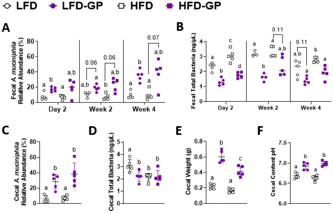
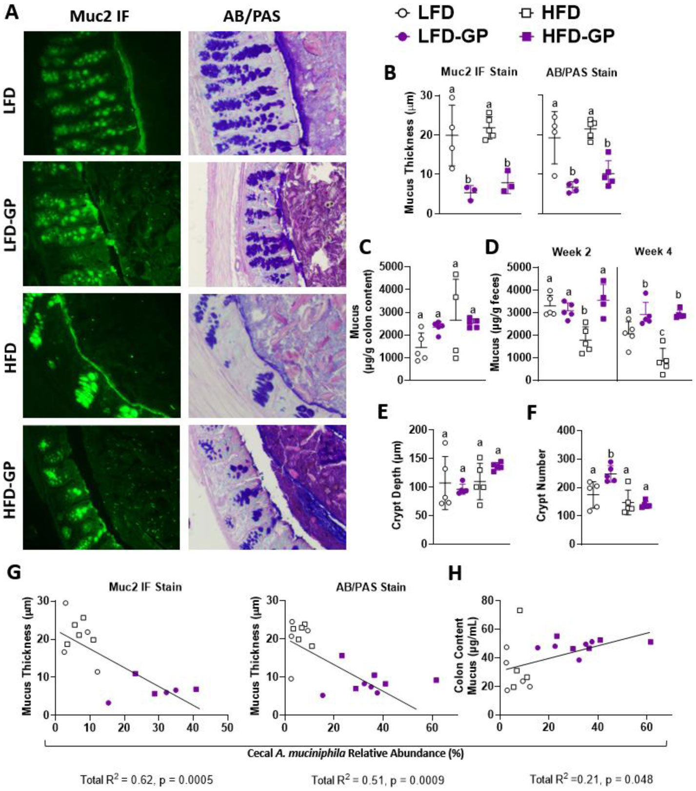
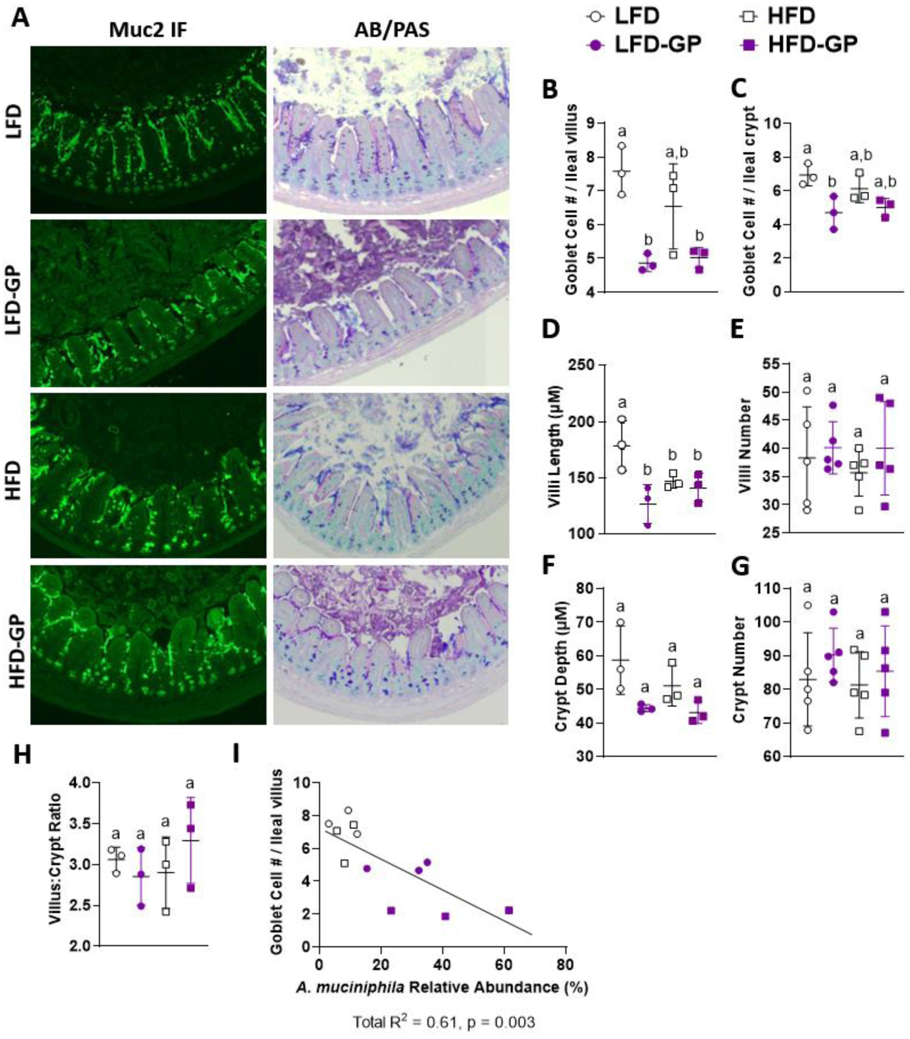
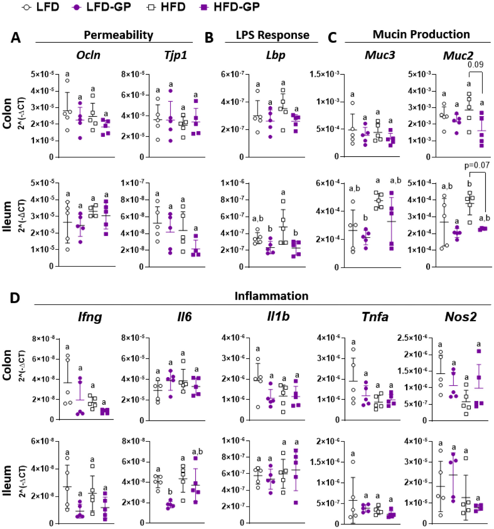
A healthy gastrointestinal tract functions as a highly selective barrier, allowing the absorption of nutrients and metabolites while preventing gut bacteria and other xenobiotic compounds from entering host circulation and tissues. The intestinal epithelium and intestinal mucus provide a physical first line of defense against resident microbes, pathogens and xenotoxic compounds. Prior studies have indicated that the gut microbe Akkermansia muciniphila, a mucin-metabolizer, can stimulate intestinal mucin thickness to improve gut barrier integrity. Grape polyphenol (GP) extracts rich in B-type proanthocyanidin (PAC) compounds have been found to increase the relative abundance of A. muciniphila, suggesting that PACs alter the gut microbiota to support a healthy gut barrier. To further investigate the effect of GPs on the gut barrier and A. muciniphila, male C57BL/6 mice were fed a high-fat diet (HFD) or low-fat diet (LFD) with or without 1% GPs (HFD-GP, LFD-GP) for 12 weeks. Compared to the mice fed unsupplemented diets, GP-supplemented mice showed increased relative abundance of fecal and cecal A. muciniphila, a reduction in total bacteria, a diminished colon mucus layer and increased fecal mucus content. GP supplementation also reduced the presence of goblet cells regardless of dietary fat. Compared to the HFD group, ileal gene expression of lipopolysaccharide (LPS)-binding protein (Lbp), an acute-phase protein that promotes pro-inflammatory cytokine expression, was reduced in the HFD-GP group, suggesting reduced LPS in circulation. Despite depletion of the colonic mucus layer, markers of inflammation (Ifng, Il1b, Tnfa, and Nos2) were similar among the four groups, with the exception that ileal Il6 mRNA levels were lower in the LFD-GP group compared to the LFD group. Our findings suggest that the GP-induced increase in A. muciniphila promotes redistribution of the intestinal mucus layer to the intestinal lumen, and that the GP-induced decrease in total bacteria results in a less inflammatory intestinal milieu.

Citation: Esther Mezhibovsky, Yue Wu, Fiona G. Bawagan, Kevin M. Tveter, Samantha Szeto, Diana Roopchand. Impact of grape polyphenols on Akkermansia muciniphila and the gut barrier[J]. AIMS Microbiology, 2022, 8(4): 544-565. doi: 10.3934/microbiol.2022035
A healthy gastrointestinal tract functions as a highly selective barrier, allowing the absorption of nutrients and metabolites while preventing gut bacteria and other xenobiotic compounds from entering host circulation and tissues. The intestinal epithelium and intestinal mucus provide a physical first line of defense against resident microbes, pathogens and xenotoxic compounds. Prior studies have indicated that the gut microbe Akkermansia muciniphila, a mucin-metabolizer, can stimulate intestinal mucin thickness to improve gut barrier integrity. Grape polyphenol (GP) extracts rich in B-type proanthocyanidin (PAC) compounds have been found to increase the relative abundance of A. muciniphila, suggesting that PACs alter the gut microbiota to support a healthy gut barrier. To further investigate the effect of GPs on the gut barrier and A. muciniphila, male C57BL/6 mice were fed a high-fat diet (HFD) or low-fat diet (LFD) with or without 1% GPs (HFD-GP, LFD-GP) for 12 weeks. Compared to the mice fed unsupplemented diets, GP-supplemented mice showed increased relative abundance of fecal and cecal A. muciniphila, a reduction in total bacteria, a diminished colon mucus layer and increased fecal mucus content. GP supplementation also reduced the presence of goblet cells regardless of dietary fat. Compared to the HFD group, ileal gene expression of lipopolysaccharide (LPS)-binding protein (Lbp), an acute-phase protein that promotes pro-inflammatory cytokine expression, was reduced in the HFD-GP group, suggesting reduced LPS in circulation. Despite depletion of the colonic mucus layer, markers of inflammation (Ifng, Il1b, Tnfa, and Nos2) were similar among the four groups, with the exception that ileal Il6 mRNA levels were lower in the LFD-GP group compared to the LFD group. Our findings suggest that the GP-induced increase in A. muciniphila promotes redistribution of the intestinal mucus layer to the intestinal lumen, and that the GP-induced decrease in total bacteria results in a less inflammatory intestinal milieu.

| [1] |
Ghosh SS, Wang J, Yannie PJ, et al. (2020) Intestinal barrier dysfunction, LPS translocation, and disease development. J Endocr Soc 4: bvz039. https://doi.org/10.1210/jendso/bvz039 
|
| [2] |
Paone P, Cani PD (2020) Mucus barrier, mucins and gut microbiota: the expected slimy partners?. Gut 69: 2232-2243. https://doi.org/10.1136/gutjnl-2020-322260
|
| [3] |
Ashida H, Ogawa M, Kim M, et al. (2011) Bacteria and host interactions in the gut epithelial barrier. Nat Chem Biol 8: 36-45. https://doi.org/10.1038/nchembio.741
|
| [4] |
Van der Sluis M, De Koning BA, De Bruijn AC, et al. (2006) Muc2-deficient mice spontaneously develop colitis, indicating that MUC2 is critical for colonic protection. Gastroenterology 131: 117-129. https://doi.org/10.1053/j.gastro.2006.04.020
|
| [5] |
Bergstrom KS, Kissoon-Singh V, Gibson DL, et al. (2010) Muc2 protects against lethal infectious colitis by disassociating pathogenic and commensal bacteria from the colonic mucosa. PLoS Pathog 6: e1000902. https://doi.org/10.1371/journal.ppat.1000902
|
| [6] |
Johansson ME, Larsson JM, Hansson GC (2011) The two mucus layers of colon are organized by the MUC2 mucin, whereas the outer layer is a legislator of host-microbial interactions. Proc Natl Acad Sci USA 108: 4659-4665. https://doi.org/10.1073/pnas.1006451107
|
| [7] |
Kamphuis JBJ, Mercier-Bonin M, Eutamène H, et al. (2017) Mucus organisation is shaped by colonic content; a new view. Sci Rep 7: 8527. https://doi.org/10.1038/s41598-017-08938-3
|
| [8] |
Derrien M, Collado MC, Ben-Amor K, et al. (2008) The Mucin degrader Akkermansia muciniphila is an abundant resident of the human intestinal tract. Appl Environ Microbiol 74: 1646-1648. https://doi.org/10.1128/AEM.01226-07
|
| [9] |
Johansson MEV, Phillipson M, Petersson J, et al. (2008) The inner of the two Muc2 mucin-dependent mucus layers in colon is devoid of bacteria. Proc Nat Acad Sci 105: 15064-15069. https://doi.org/10.1073/pnas.0803124105
|
| [10] |
Pédron T, Mulet C, Dauga C, et al. (2012) A crypt-specific core microbiota resides in the mouse colon. mBio 3: e00116-12. https://doi.org/10.1128/mBio.00116-12
|
| [11] |
Swidsinski A, Loening-Baucke V, Lochs H, et al. (2005) Spatial organization of bacterial flora in normal and inflamed intestine: a fluorescence in situ hybridization study in mice. World J Gastroenterol 11: 1131-1140. https://doi.org/10.3748/wjg.v11.i8.1131
|
| [12] |
Swidsinski A, Weber J, Loening-Baucke V, et al. (2005) Spatial organization and composition of the mucosal flora in patients with inflammatory bowel disease. J Clin Microbiol 43: 3380-3389. https://doi.org/10.1128/JCM.43.7.3380-3389.2005
|
| [13] |
Round JL, Lee SM, Li J, et al. (2011) The Toll-like receptor 2 pathway establishes colonization by a commensal of the human microbiota. Science 332: 974-977. https://doi.org/10.1126/science.1206095
|
| [14] |
Lee SM, Donaldson GP, Mikulski Z, et al. (2013) Bacterial colonization factors control specificity and stability of the gut microbiota. Nature 501: 426-429. https://doi.org/10.1038/nature12447
|
| [15] |
Ulluwishewa D, Anderson RC, McNabb WC, et al. (2011) Regulation of tight junction permeability by intestinal bacteria and dietary components. J Nutr 141: 769-776. https://doi.org/10.3945/jn.110.135657
|
| [16] |
Cani PD, Bibiloni R, Knauf C, et al. (2008) Changes in gut microbiota control metabolic endotoxemia-induced inflammation in high-fat diet-induced obesity and diabetes in mice. Diabetes 57: 1470-1481. https://doi.org/10.2337/db07-1403
|
| [17] |
Suzuki T, Hara H (2010) Dietary fat and bile juice, but not obesity, are responsible for the increase in small intestinal permeability induced through the suppression of tight junction protein expression in LETO and OLETF rats. Nutr Metab (Lond) 7: 19. https://doi.org/10.1186/1743-7075-7-19
|
| [18] |
Stenman LK, Holma R, Korpela R (2012) High-fat-induced intestinal permeability dysfunction associated with altered fecal bile acids. World J Gastroenterol 18: 923-929. https://doi.org/10.3748/wjg.v18.i9.923
|
| [19] |
Araújo JR, Tomas J, Brenner C, et al. (2017) Impact of high-fat diet on the intestinal microbiota and small intestinal physiology before and after the onset of obesity. Biochimie 141: 97-106. https://doi.org/10.1016/j.biochi.2017.05.019
|
| [20] |
Cani PD, Amar J, Iglesias MA, et al. (2007) Metabolic endotoxemia initiates obesity and insulin resistance. Diabetes 56: 1761-1772. https://doi.org/10.2337/db06-1491
|
| [21] |
Ghanim H, Abuaysheh S, Sia CL, et al. (2009) Increase in plasma endotoxin concentrations and the expression of Toll-like receptors and suppressor of cytokine signaling-3 in mononuclear cells after a high-fat, high-carbohydrate meal: implications for insulin resistance. Diabetes Care 32: 2281-2287. https://doi.org/10.2337/dc09-0979
|
| [22] |
Ryu JK, Kim SJ, Rah SH, et al. (2017) Reconstruction of LPS transfer cascade reveals structural determinants within LBP, CD14, and TLR4-MD2 for efficient LPS recognition and transfer. Immunity 46: 38-50. https://doi.org/10.1016/j.immuni.2016.11.007
|
| [23] |
Andrews C, McLean MH, Durum SK (2018) Cytokine tuning of intestinal epithelial function. Front Immunol 9: 1270. https://doi.org/10.3389/fimmu.2018.01270
|
| [24] |
Matziouridou C, Rocha SDC, Haabeth OA, et al. (2018) iNOS- and NOX1-dependent ROS production maintains bacterial homeostasis in the ileum of mice. Mucosal Immunol 11: 774-784. https://doi.org/10.1038/mi.2017.106
|
| [25] | Rohr MW, Narasimhulu CA, Rudeski-Rohr TA, et al. (2020) Negative effects of a high-fat diet on intestinal permeability: A review. Adv Nutr 11: 77-91. https://doi.org/10.1093/advances/nmz061 |
| [26] |
Everard A, Belzer C, Geurts L, et al. (2013) Cross-talk between Akkermansia muciniphila and intestinal epithelium controls diet-induced obesity. Proc Natl Acad Sci USA 110: 9066-9071. https://doi.org/10.1073/pnas.1219451110
|
| [27] |
Roopchand DE, Carmody RN, Kuhn P, et al. (2015) Dietary polyphenols promote growth of the gut bacterium Akkermansia muciniphila and attenuate high-fat diet-induced metabolic syndrome. Diabetes 64: 2847-2858. https://doi.org/10.2337/db14-1916
|
| [28] |
Ottman N, Reunanen J, Meijerink M, et al. (2017) Pili-like proteins of Akkermansia muciniphila modulate host immune responses and gut barrier function. PLoS One 12: e0173004. https://doi.org/10.1371/journal.pone.0173004
|
| [29] |
Schneeberger M, Everard A, Gómez-Valadés AG, et al. (2015) Akkermansia muciniphila inversely correlates with the onset of inflammation, altered adipose tissue metabolism and metabolic disorders during obesity in mice. Sci Rep 5: 16643. https://doi.org/10.1038/srep16643
|
| [30] |
Dao MC, Everard A, Aron-Wisnewsky J, et al. (2016) Akkermansia muciniphila and improved metabolic health during a dietary intervention in obesity: relationship with gut microbiome richness and ecology. Gut 65: 426-436. https://doi.org/10.1136/gutjnl-2014-308778
|
| [31] |
Bi J, Liu S, Du G, et al. (2016) Bile salt tolerance of Lactococcus lactis is enhanced by expression of bile salt hydrolase thereby producing less bile acid in the cells. Biotechnol Lett 38: 659-665. https://doi.org/10.1007/s10529-015-2018-7
|
| [32] |
Anhê FF, Roy D, Pilon G, et al. (2015) A polyphenol-rich cranberry extract protects from diet-induced obesity, insulin resistance and intestinal inflammation in association with increased Akkermansia spp. population in the gut microbiota of mice. Gut 64: 872-883. https://doi.org/10.1136/gutjnl-2014-307142
|
| [33] |
Anhê FF, Nachbar RT, Varin TV, et al. (2019) Treatment with camu camu (Myrciaria dubia) prevents obesity by altering the gut microbiota and increasing energy expenditure in diet-induced obese mice. Gut 68: 453-464. https://doi.org/10.1136/gutjnl-2017-315565
|
| [34] |
Depommier C, Everard A, Druart C, et al. (2019) Supplementation with Akkermansia muciniphila in overweight and obese human volunteers: a proof-of-concept exploratory study. Nat Med 25: 1096-1103. https://doi.org/10.1038/s41591-019-0495-2
|
| [35] |
de la Cuesta-Zuluaga J, Mueller NT, Corrales-Agudelo V, et al. (2016) Metformin is associated with higher relative abundance of mucin-degrading Akkermansia muciniphila and several short-chain fatty acid–producing microbiota in the gut. Diabetes Care 40: 54-62. https://doi.org/10.2337/dc16-1324
|
| [36] |
Wu H, Esteve E, Tremaroli V, et al. (2017) Metformin alters the gut microbiome of individuals with treatment-naive type 2 diabetes, contributing to the therapeutic effects of the drug. Nat Med 23: 850-858. https://doi.org/10.1038/nm.4345
|
| [37] |
Shin NR, Lee JC, Lee HY, et al. (2014) An increase in the Akkermansia spp. population induced by metformin treatment improves glucose homeostasis in diet-induced obese mice. Gut 63: 727-735. https://doi.org/10.1136/gutjnl-2012-303839
|
| [38] |
Ganesh BP, Klopfleisch R, Loh G, et al. (2013) Commensal Akkermansia muciniphila exacerbates gut inflammation in Salmonella Typhimurium-infected gnotobiotic mice. PLoS One 8: e74963. https://doi.org/10.1371/journal.pone.0074963
|
| [39] |
Han Y, Song M, Gu M, et al. (2019) Dietary intake of whole strawberry inhibited colonic inflammation in dextran-sulfate-sodium-treated mice via restoring immune homeostasis and alleviating gut microbiota dysbiosis. J Agric Food Chem 67: 9168-9177. https://doi.org/10.1021/acs.jafc.8b05581
|
| [40] |
Lukovac S, Belzer C, Pellis L, et al. (2014) Differential modulation by Akkermansia muciniphila and Faecalibacterium prausnitzii of host peripheral lipid metabolism and histone acetylation in mouse gut organoids. mBio 5: e01438-14. https://doi.org/10.1128/mBio.01438-14
|
| [41] |
Plovier H, Everard A, Druart C, et al. (2017) A purified membrane protein from Akkermansia muciniphila or the pasteurized bacterium improves metabolism in obese and diabetic mice. Nat Med 23: 107-113. https://doi.org/10.1038/nm.4236
|
| [42] |
Zhang L, Carmody RN, Kalariya HM, et al. (2018) Grape proanthocyanidin-induced intestinal bloom of Akkermansia muciniphila is dependent on its baseline abundance and precedes activation of host genes related to metabolic health. J Nutr Biochem 56: 142-151. https://doi.org/10.1016/j.jnutbio.2018.02.009
|
| [43] |
Tveter KM, Villa-Rodriguez JA, Cabales AJ, et al. (2020) Polyphenol-induced improvements in glucose metabolism are associated with bile acid signaling to intestinal farnesoid X receptor. BMJ Open Diabetes Res Care 8. https://doi.org/10.1136/bmjdrc-2020-001386
|
| [44] |
Mezhibovsky E, Knowles KA, He Q, et al. (2021) Grape polyphenols attenuate diet-induced obesity and hepatic steatosis in mice in association with reduced butyrate and increased markers of intestinal carbohydrate oxidation. Front Nutr 8: 675267. https://doi.org/10.3389/fnut.2021.675267
|
| [45] |
Ezzat-Zadeh Z, Henning SM, Yang J, et al. (2021) California strawberry consumption increased the abundance of gut microorganisms related to lean body weight, health and longevity in healthy subjects. Nutr Res 85: 60-70. https://doi.org/10.1016/j.nutres.2020.12.006
|
| [46] | Gao X, Xie Q, Kong P, et al. (2018) Polyphenol- and caffeine-rich postfermented Pu-erh tea improves diet-induced metabolic syndrome by remodeling intestinal homeostasis in mice. Infect Immun 86. https://doi.org/10.1128/IAI.00601-17 |
| [47] |
Régnier M, Rastelli M, Morissette A, et al. (2020) Rhubarb supplementation prevents diet-induced obesity and diabetes in association with increased Akkermansia muciniphila in mice. Nutrients 12. https://doi.org/10.3390/nu12102932
|
| [48] |
Mezhibovsky E, Knowles KA, He Q, et al. (2021) Grape polyphenols attenuate diet-induced obesity and hepatic steatosis in mice in association with reduced butyrate and increased markers of intestinal carbohydrate oxidation. Front Nutr 8: 1-14. https://doi.org/10.3389/fnut.2021.675267
|
| [49] |
Villa-Rodriguez JA, Ifie I, Gonzalez-Aguilar GA, et al. (2019) The gastrointestinal tract as prime site for cardiometabolic protection by dietary polyphenols. Adv Nutr 10: 999-1011. https://doi.org/10.1093/advances/nmz038
|
| [50] |
Johansson ME, Hansson GC (2012) Preservation of mucus in histological sections, immunostaining of mucins in fixed tissue, and localization of bacteria with FISH. Methods Mol Biol 842: 229-235. https://doi.org/10.1007/978-1-61779-513-8_13
|
| [51] |
Bovee-Oudenhoven IM, Termont DS, Heidt PJ, et al. (1997) Increasing the intestinal resistance of rats to the invasive pathogen Salmonella enteritidis: additive effects of dietary lactulose and calcium. Gut 40: 497. https://doi.org/10.1136/gut.40.4.497
|
| [52] |
Savage DC, Dubos R (1968) Alterations in the mouse cecum and its flora produced by antibacterial drugs. J Exp Med 128: 97-110. https://doi.org/10.1084/jem.128.1.97
|
| [53] |
Van Herreweghen F, Van den Abbeele P, De Mulder T, et al. (2017) In vitro colonisation of the distal colon by Akkermansia muciniphila is largely mucin and pH dependent. Benef Microbes 8: 81-96. https://doi.org/10.3920/BM2016.0013
|
| [54] |
Sangiorgi E, Capecchi MR (2008) Bmi1 is expressed in vivo in intestinal stem cells. Nat Genet 40: 915-920. https://doi.org/10.1038/ng.165
|
| [55] |
Vetushchi A, Sferra R, Caprilli R, et al. (2002) Increased proliferation and apoptosis of colonic epithelial cells in dextran sulfate sodium-induced colitis in rats. Dig Dis Sci 47: 1447-1457. https://doi.org/10.1023/A:1015931128583
|
| [56] |
Dinh CH, Yu Y, Szabo A, et al. (2016) Bardoxolone methyl prevents high-fat diet-induced colon inflammation in mice. J Histochem Cytochem 64: 237-255. https://doi.org/10.1369/0022155416631803
|
| [57] | Xie Y, Ding F, Di W, et al. (2020) Impact of a highfat diet on intestinal stem cells and epithelial barrier function in middleaged female mice. Mol Med Rep 21: 1133-1144. https://doi.org/10.3892/mmr.2020.10932 |
| [58] |
John Totafurno MB, Cheng Hazel (1987) The crypt cycle: Crypt and villus production in the adult intestinal epithelium. Biophys J 52: 279-294. https://doi.org/10.1016/S0006-3495(87)83215-0
|
| [59] |
Sainsbury A, Goodlad RA, Perry SL, et al. (2008) Increased colorectal epithelial cell proliferation and crypt fission associated with obesity and roux-en-Y gastric bypass. Cancer Epidemiol Biomarkers Prev 17: 1401-1410. https://doi.org/10.1158/1055-9965.EPI-07-2874
|
| [60] | Shahbazi P, Nematollahi A, Arshadi S, et al. (2021) The protective effect of Artemisia spicigera ethanolic extract against Cryptosporidium parvum infection in immunosuppressed mice. Iran J Parasitol 16: 279-288. https://doi.org/10.18502/ijpa.v16i2.6318 |
| [61] |
Argenzio RA, Liacos JA, Levy ML, et al. (1990) Villous atrophy, crypt hyperplasia, cellular infiltration, and impaired glucose-NA absorption in enteric cryptosporidiosis of pigs. Gastroenterology 98: 1129-1140. https://doi.org/10.1016/0016-5085(90)90325-U
|
| [62] |
Liu X, Lu L, Yao P, et al. (2014) Lipopolysaccharide binding protein, obesity status and incidence of metabolic syndrome: a prospective study among middle-aged and older Chinese. Diabetologia 57: 1834-1841. https://doi.org/10.1007/s00125-014-3288-7
|
| [63] |
Moreno-Navarrete JM, Ortega F, Serino M, et al. (2012) Circulating lipopolysaccharide-binding protein (LBP) as a marker of obesity-related insulin resistance. Int J Obes (Lond) 36: 1442-1449. https://doi.org/10.1038/ijo.2011.256
|
| [64] |
Birchenough GM, Nyström EE, Johansson ME, et al. (2016) A sentinel goblet cell guards the colonic crypt by triggering Nlrp6-dependent Muc2 secretion. Science 352: 1535-1542. https://doi.org/10.1126/science.aaf7419
|
| [65] |
Visioli F (2015) Xenobiotics and human health: A new view of their pharma-nutritional role. PharmaNutrition 3: 60-64. https://doi.org/10.1016/j.phanu.2015.04.001
|
| [66] | Lambert MGSaGH.Xenobiotic-induced hepatotoxicity: mechanisms of liver injury and methods of monitoring hepatic function. Clin Chem (1997) 43: 1512-1525. https://doi.org/10.1093/clinchem/43.8.1512 |
| [67] |
Hall DM, Sattler GL, Sattler CA, et al. (2001) Aging lowers steady-state antioxidant enzyme and stress protein expression in primary hepatocytes. J Gerontol Biol Sci 56A: B259-B267. https://doi.org/10.1093/gerona/56.6.B259
|
| [68] |
Liang H, Jiang F, Cheng R, et al. (2021) A high-fat diet and high-fat and high-cholesterol diet may affect glucose and lipid metabolism differentially through gut microbiota in mice. Exp Anim 70: 73-83. https://doi.org/10.1538/expanim.20-0094
|
| [69] |
Reagan WJ, Yang RZ, Park S, et al. (2012) Metabolic adaptive ALT isoenzyme response in livers of C57/BL6 mice treated with dexamethasone. Toxicol Pathol 40: 1117-1127. https://doi.org/10.1177/0192623312447550
|
| [70] |
Kuhn P, Kalariya HM, Poulev A, et al. (2018) Grape polyphenols reduce gut-localized reactive oxygen species associated with the development of metabolic syndrome in mice. PLoS One 13: e0198716. https://doi.org/10.1371/journal.pone.0198716
|
| [71] |
Dubourg G, Lagier JC, Armougom F, et al. (2013) High-level colonisation of the human gut by Verrucomicrobia following broad-spectrum antibiotic treatment. Int J Antimicrob Agents 41: 149-155. https://doi.org/10.1016/j.ijantimicag.2012.10.012
|
| [72] | Chen CY, Hsu KC, Yeh HY, et al. (2020) Visualizing the effects of antibiotics on the mouse colonic mucus layer. Ci Ji Yi Xue Za Zhi 32: 145-153. https://doi.org/10.4103/tcmj.tcmj_70_19 |
| [73] |
Taira T, Yamaguchi S, Takahashi A, et al. (2015) Dietary polyphenols increase fecal mucin and immunoglobulin A and ameliorate the disturbance in gut microbiota caused by a high fat diet. J Clin Biochem Nutr 57: 212-216. https://doi.org/10.3164/jcbn.15-15
|
| [74] | Forgie AJ, Ju T, Tollenaar SL, et al. (2022) Phytochemical-induced mucin accumulation in the gastrointestinal lumen is independent of the microbiota. bioRxiv : 2022.2003.2011.483917. https://doi.org/10.1101/2022.03.11.483917 |
| [75] |
Davies HS, Pudney PDA, Georgiades P, et al. (2014) Reorganisation of the salivary mucin network by dietary components: Insights from green tea polyphenols. PLOS One 9: e108372. https://doi.org/10.1371/journal.pone.0108372
|
| [76] |
Tveter KM, Villa JA, Cabales AJ, et al. (2020) Polyphenol-induced improvements in glucose metabolism are associated with bile acid signaling to intestinal farnesoid X receptor. BMJ Open Diabetes Res Care 8: 1-12. https://doi.org/10.1136/bmjdrc-2020-001386
|
| [77] |
Hansen CH, Krych L, Nielsen DS, et al. (2012) Early life treatment with vancomycin propagates Akkermansia muciniphila and reduces diabetes incidence in the NOD mouse. Diabetologia 55: 2285-2294. https://doi.org/10.1007/s00125-012-2564-7
|
| [78] |
Petersson J, Schreiber O, Hansson GC, et al. (2011) Importance and regulation of the colonic mucus barrier in a mouse model of colitis. Am J Physiol Gastrointest Liver Physiol 300: G327-333. https://doi.org/10.1152/ajpgi.00422.2010
|
| [79] | Mack DR, Michail S, Wei S, et al. (1999) Probiotics inhibit enteropathogenic E. coli adherence in vitro by inducing intestinal mucin gene expression. Am J Physiol 276: G941-950. https://doi.org/10.1152/ajpgi.1999.276.4.G941 |
| [80] |
Mack DR, Ahrne S, Hyde L, et al. (2003) Extracellular MUC3 mucin secretion follows adherence of Lactobacillus strains to intestinal epithelial cells in vitro. Gut 52: 827-833. https://doi.org/10.1136/gut.52.6.827
|
| [81] | Lazlo Szentkuti M-LE (1998) Comparative lectin-histochemistry on the pre-epithelial mucus layer in the distal colon of conventional and germ-free rats. Comp Biochem Physiol 119A: 379-386. https://doi.org/10.1016/S1095-6433(97)00434-0 |
| [82] |
Umesaki Y, Tohyama K, Mutai M (1982) Biosynthesis of microvillus membrane-associated glycoproteins of small intestinal epithelial cells in germ-free and conventionalized mice. J Biochem 92: 373-379. https://doi.org/10.1093/oxfordjournals.jbchem.a133943
|
| [83] |
Kandori H, Hirayama K, Takeda M, et al. (1996) Histochemical, lectin-histochemical and morphometrical characteristics of intestinal goblet cells of germfree and conventional mice. Exp Anim 45: 155-160. https://doi.org/10.1538/expanim.45.155
|
| [84] |
Comelli EM, Simmering R, Faure M, et al. (2008) Multifaceted transcriptional regulation of the murine intestinal mucus layer by endogenous microbiota. Genomics 91: 70-77. https://doi.org/10.1016/j.ygeno.2007.09.006
|
| [85] |
Wlodarska M, Willing B, Keeney KM, et al. (2011) Antibiotic treatment alters the colonic mucus layer and predisposes the host to exacerbated Citrobacter rodentium-induced colitis. Infect Immun 79: 1536-1545. https://doi.org/10.1128/IAI.01104-10
|
 microbiol-08-04-035-s001.pdf microbiol-08-04-035-s001.pdf |
 |
Figures(4)

Esther Mezhibovsky, Yue Wu, Fiona G. Bawagan, Kevin M. Tveter, Samantha Szeto, Diana Roopchand. Impact of grape polyphenols on Akkermansia muciniphila and the gut barrier[J]. AIMS Microbiology, 2022, 8(4): 544-565. doi: 10.3934/microbiol.2022035


 DownLoad: