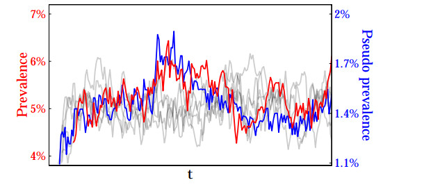
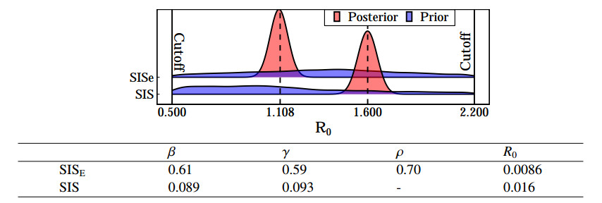
This paper offers a qualitative insight into the convergence of Bayesian parameter inference in a setup which mimics the modeling of the spread of a disease with associated disease measurements. Specifically, we are interested in the Bayesian model's convergence with increasing amounts of data under measurement limitations. Depending on how weakly informative the disease measurements are, we offer a kind of 'best case' as well as a 'worst case' analysis where, in the former case, we assume that the prevalence is directly accessible, while in the latter that only a binary signal corresponding to a prevalence detection threshold is available. Both cases are studied under an assumed so-called linear noise approximation as to the true dynamics. Numerical experiments test the sharpness of our results when confronted with more realistic situations for which analytical results are unavailable.
Citation: Samuel Bronstein, Stefan Engblom, Robin Marin. Bayesian inference in epidemics: linear noise analysis[J]. Mathematical Biosciences and Engineering, 2023, 20(2): 4128-4152. doi: 10.3934/mbe.2023193
This paper offers a qualitative insight into the convergence of Bayesian parameter inference in a setup which mimics the modeling of the spread of a disease with associated disease measurements. Specifically, we are interested in the Bayesian model's convergence with increasing amounts of data under measurement limitations. Depending on how weakly informative the disease measurements are, we offer a kind of 'best case' as well as a 'worst case' analysis where, in the former case, we assume that the prevalence is directly accessible, while in the latter that only a binary signal corresponding to a prevalence detection threshold is available. Both cases are studied under an assumed so-called linear noise approximation as to the true dynamics. Numerical experiments test the sharpness of our results when confronted with more realistic situations for which analytical results are unavailable.

| [1] | M. J. Keeling, P. Rohani, Modeling Infectious Diseases in Humans and Animals, Princeton University Press, 2011. https://doi.org/10.1086/591197 |
| [2] |
T. McKinley, A. R. Cook, R. Deardon, Inference in epidemic models without likelihoods, Int. J. Biostat., 5 (2009). https://doi.org/10.2202/1557-4679.1171 doi: 10.2202/1557-4679.1171

|
| [3] | H. Andersson, T. Britton, Stochastic Epidemic Models and Their Statistical Analysis, Springer Science & Business Media, 151 (2012). https://doi.org/10.1007/978-1-4612-1158-7 |
| [4] |
S. Eubank, H. Guclu, V. A. Kumar, M. V. Marathe, A. Srinivasan, Z. Toroczkai, et al., Modelling disease outbreaks in realistic urban social networks, Nature, 429 (2004), 180–184. https://doi.org/10.1038/nature02541 doi: 10.1038/nature02541
|
| [5] |
N. M. Ferguson, D. A. Cummings, S. Cauchemez, C. Fraser, S. Riley, A. Meeyai, et al., Strategies for containing an emerging influenza pandemic in southeast Asia, Nature, 437 (2005), 209–214. https://doi.org/10.1038/nature04017 doi: 10.1038/nature04017
|
| [6] |
D. Balcan, V. Colizza, B. Gonçalves, H. Hu, J. J. Ramasco, A. Vespignani, Multiscale mobility networks and the spatial spreading of infectious diseases, Proc. Natl. Acad. Sci. USA, 106 (2009), 21484–21489. https://doi.org/10.1073/pnas.0906910106 doi: 10.1073/pnas.0906910106
|
| [7] |
S. Merler, M. Ajelli, A. Pugliese, N. M. Ferguson, Determinants of the spatiotemporal dynamics of the 2009 H1N1 pandemic in Europe: implications for real-time modelling, PLoS Comput. Biol., 7 (2011), e1002205. https://doi.org/10.1371/journal.pcbi.1002205 doi: 10.1371/journal.pcbi.1002205
|
| [8] |
E. Brooks-Pollock, G. O. Roberts, M. J. Keeling, A dynamic model of bovine tuberculosis spread and control in Great Britain, Nature, 511 (2014), 228–231. https://doi.org/10.1038/nature13529 doi: 10.1038/nature13529
|
| [9] |
J. Stehlé, N. Voirin, A. Barrat, C. Cattuto, V. Colizza, L. Isella, et al., Simulation of an SEIR infectious disease model on the dynamic contact network of conference attendees, BMC Med., 9 (2011), 87. https://doi.org/10.1186/1741-7015-9-87 doi: 10.1186/1741-7015-9-87
|
| [10] |
P. Bajardi, A. Barrat, L. Savini, V. Colizza, Optimizing surveillance for livestock disease spreading through animal movements, J. R. Soc. Interface, 9 (2012), 2814–2825. https://doi.org/10.1186/1741-7015-9-87 doi: 10.1186/1741-7015-9-87
|
| [11] |
M. Salathé, M. Kazandjieva, J. W. Lee, P. Levis, M. W. Feldman, J. H. Jones, A high-resolution human contact network for infectious disease transmission, Proc. Natl. Acad. Sci. USA, 107 (2010), 22020–22025. https://doi.org/10.1073/pnas.1009094108 doi: 10.1073/pnas.1009094108
|
| [12] |
T. Obadia, R. Silhol, L. Opatowski, L. Temime, J. Legrand, A. C. M. Thiéaut, et al., Detailed contact data and the dissemination of Staphylococcus aureus in hospitals, PLoS Comput. Biol., 11 (2015), e1004170. https://doi.org/10.1371/journal.pcbi.1004170 doi: 10.1371/journal.pcbi.1004170
|
| [13] |
D. J. Toth, M. Leecaster, W. B. Pettey, A. V. Gundlapalli, H. Gao, J. J. Rainey, et al., The role of heterogeneity in contact timing and duration in network models of influenza spread in schools, J. R. Soc. Interface, 12 (2015), 20150279. https://doi.org/10.1098/rsif.2015.0279 doi: 10.1098/rsif.2015.0279
|
| [14] |
Q. Zhang, K. Sun, M. Chinazzi, A. P. y Piontti, N. E. Dean, D. P. Rojas, et al., Spread of Zika virus in the Americas, Proc. Natl. Acad. Sci. USA, 114 (2017), E4334–E4343. https://doi.org/10.1073/pnas.1620161114 doi: 10.1073/pnas.1620161114
|
| [15] |
Q. H. Liu, M. Ajelli, A. Aleta, S. Merler, Y. Moreno, A. Vespignani, Measurability of the epidemic reproduction number in data-driven contact networks, Proc. Natl. Acad. Sci. USA, 115 (2018), 12680–12685. https://doi.org/10.1073/pnas.1811115115 doi: 10.1073/pnas.1811115115
|
| [16] |
S. Widgren, S. Engblom, U. Emanuelson, A. Lindberg, Spatio-temporal modelling of verotoxigenic Escherichia coli O157 in cattle in Sweden: exploring options for control, Vet. Res., 49 (2018). https://doi.org/10.1186/s13567-018-0574-2 doi: 10.1186/s13567-018-0574-2
|
| [17] | T. Söderström, P. Stoica, System Identification, Prentice-Hall International, 1989. |
| [18] |
G. Fournié, A. Waret-Szkuta, A. Camacho, L. M. Yigezu, D. U. Pfeiffer, F. Roger, A dynamic model of transmission and elimination of peste des petits ruminants in Ethiopia, Proc. Natl. Acad. Sci. USA, 115 (2018), 8454–8459. https://doi.org/10.1073/pnas.1711646115 doi: 10.1073/pnas.1711646115
|
| [19] |
S. Engblom, R. Eriksson, S. Widgren, Bayesian epidemiological modeling over high-resolution network data, Epidemics, 32 (2020), 100399. https://doi.org/10.1016/j.epidem.2020.100399 doi: 10.1016/j.epidem.2020.100399
|
| [20] |
X. Shen, L. Wasserman, Rates of convergence of posterior distributions, Ann. Stat., 29 (2001), 687–714. https://doi.org/10.1214/aos/1009210686 doi: 10.1214/aos/1009210686
|
| [21] |
A. M. Stuart, Inverse problems: a Bayesian perspective, Acta Numer., 19 (2010), 451–559. https://doi.org/10.1017/S0962492910000061 doi: 10.1017/S0962492910000061
|
| [22] |
A. Stuart, A. Teckentrup, Posterior consistency for Gaussian process approximations of Bayesian posterior distributions, Math. Comput., 87 (2018), 721–753. https://doi.org/10.1090/mcom/3244 doi: 10.1090/mcom/3244
|
| [23] |
J. Latz, On the well-posedness of Bayesian inverse problems, SIAM/ASA J. Uncert. Quant., 8 (2020), 451–482. https://doi.org/10.1137/19M1247176 doi: 10.1137/19M1247176
|
| [24] |
H. Owhadi, C. Scovel, T. Sullivan, On the brittleness of Bayesian inference, SIAM Rev., 57 (2015), 566–582. https://doi.org/10.1137/130938633 doi: 10.1137/130938633
|
| [25] |
B. Sprungk, On the local Lipschitz stability of Bayesian inverse problems, Inverse Probl., 36 (2020), 055015. https://doi.org/10.1088/1361-6420/ab6f43 doi: 10.1088/1361-6420/ab6f43
|
| [26] |
A. Galani, R. Aalizadeh, M. Kostakis, A. Markou, N. Alygizakis, T. Lytras, et al., SARS-CoV-2 wastewater surveillance data can predict hospitalizations and ICU admissions, Sci. Total Environ., 804 (2022), 150151. https://doi.org/10.1016/j.scitotenv.2021.150151 doi: 10.1016/j.scitotenv.2021.150151
|
| [27] |
B. Kennedy, H. Fitipaldi, U. Hammar, M. Maziarz, N. Tsereteli, N. Oskolkov, et al., App-based COVID-19 syndromic surveillance and prediction of hospital admissions in COVID Symptom Study Sweden, Nat. Commun., 13 (2022), 2110. https://doi.org/10.1038/s41467-022-29608-7 doi: 10.1038/s41467-022-29608-7
|
| [28] |
W. O. Kermack, A. G. McKendrick, A contribution to the mathematical theory of epidemics, Proc. R. Soc. Lond. A, 115 (1927), 700–721. https://doi.org/10.1098/rspa.1927.0118 doi: 10.1098/rspa.1927.0118
|
| [29] | S. Engblom, S. Widgren, Data-driven computational disease spread modeling: from measurement to parametrization and control, in Disease Modeling and Public Health: Part A, Handbook of Statistics, Chapter 11 (eds. C. R. Rao, A. S. Rao, S. Payne), Elsevier, Amsterdam, 36 (2017), 305–328. https://doi.org/10.1016/bs.host.2017.05.005 |
| [30] |
T. Britton, Stochastic epidemic models: a survey, Math. Biosci., 225 (2010), 24–35. https://doi.org/10.1016/j.mbs.2010.01.006 doi: 10.1016/j.mbs.2010.01.006
|
| [31] |
A. Gray, D. Greenhalgh, L. Hu, X. Mao, J. Pan, A stochastic differential equation SIS epidemic model, SIAM J. Appl. Math., 71 (2011), 876–902. https://doi.org/10.1137/10081856X doi: 10.1137/10081856X
|
| [32] |
G. E. Uhlenbeck, L. S. Ornstein, On the theory of the Brownian motion, Phys. Rev., 36 (1930), 823. https://doi.org/10.1103/PhysRev.36.823 doi: 10.1103/PhysRev.36.823
|
| [33] |
I. Shoji, Approximation of continuous time stochastic processes by a local linearization method, Math. Comput., 67 (1998), 287–298. https://doi.org/10.1090/S0025-5718-98-00888-6 doi: 10.1090/S0025-5718-98-00888-6
|
| [34] |
A. P. Ghosh, W. Qin, A. Roitershtein, Discrete-time Ornstein-Uhlenbeck process in a stationary dynamic environment, J. Interdiscip. Math., 19 (2016), 1–35. https://doi.org/10.1080/09720502.2013.857921 doi: 10.1080/09720502.2013.857921
|
| [35] | I. V. Basawa, B. P. Rao, Chapter 10 - Bayesian Inference for Stochastic Processes, in Statistical Inference for Stochastic Processes (eds. I. V. Basawa, B. P. Rao), Academic Press, London, 1980 (1980), 255–293. https://doi.org/10.1016/B978-0-12-080250-0.50017-8 |
| [36] |
M. Mishra, B. Prakash Rao, Rate of convergence in the Bernstein-Von Mises theorem for a class of diffusion processes, Stochastics, 22 (1987), 59–75. https://doi.org/10.1080/17442508708833467 doi: 10.1080/17442508708833467
|
| [37] |
J. Bishwal, Rates of convergence of the posterior distributions and the Bayes estimations in the Ornstein-Uhlenbeck process, Random Oper. Stoch. Equ., 8 (2000), 51–70. https://doi.org/10.1515/rose.2000.8.1.51 doi: 10.1515/rose.2000.8.1.51
|
| [38] |
D. Florens-Zmirou, Approximate discrete-time schemes for statistics of diffusion processes, Statistics: J. Theor. Appl. Stat., 20 (1989), 547–557. https://doi.org/10.1080/02331888908802205 doi: 10.1080/02331888908802205
|
| [39] |
V. Genon-Catalot, Maximum contrast estimation for diffusion processes from discrete observations, Statistics, 21 (1990), 99–116. https://doi.org/10.1080/02331889008802231 doi: 10.1080/02331889008802231
|
| [40] |
M. Kessler, Estimation of an ergodic diffusion from discrete observations. Scand. J. Stat., 24 (1997), 211–229. https://doi.org/10.1111/1467-9469.00059 doi: 10.1111/1467-9469.00059
|
| [41] | K. B. Athreya, S. N. Lahiri, Measure Theory and Probability Theory, Springer Science & Business Media, 2006. https://doi.org/10.1007/978-0-387-35434-7 |
| [42] |
E. A. Stoltenberg, N. L. Hjort, Models and inference for on-off data via clipped Ornstein-Uhlenbeck processes, Scand. J. Stat., 48 (2021), 908–929. https://doi.org/10.1111/sjos.12472 doi: 10.1111/sjos.12472
|
| [43] |
E. Slud, Clipped Gaussian processes are never M-step Markov, J. Multivariate Anal., 29 (1989), 1–14. https://doi.org/10.1016/0047-259X(89)90072-9 doi: 10.1016/0047-259X(89)90072-9
|
| [44] |
K. Joag-Dev, M. D. Perlman, L. D. Pitt, Association of normal random variables and Slepian's inequality, Ann. Probab., 11 (1983), 451–455. https://doi.org/10.1214/aop/1176993610 doi: 10.1214/aop/1176993610
|
| [45] | S. N. Ethier, T. G. Kurtz, Markov Processes: Characterization and Convergence, Wiley Series in Probability and Mathematical Statistics, John Wiley & Sons, New York, 1986. https://doi.org/10.1002/9780470316658 |
| [46] |
T. Shardlow, Modified equations for stochastic differential equations, BIT Numer. Math., 46 (2006), 111–125. https://doi.org/10.1007/s10543-005-0041-0 doi: 10.1007/s10543-005-0041-0
|
| [47] |
S. Widgren, P. Bauer, R. Eriksson, S. Engblom, SimInf: An R package for data-driven stochastic disease spread simulations, J. Stat. Software, 91 (2019), 1–42. https://doi.org/10.18637/jss.v091.i12 doi: 10.18637/jss.v091.i12
|
| [48] |
J. M. Marin, P. Pudlo, C. P. Robert, R. J. Ryder, Approximate Bayesian computational methods, Stat. Comput., 22 (2012), 1167–1180. https://doi.org/10.1007/s11222-011-9288-2 doi: 10.1007/s11222-011-9288-2
|
| [49] | S. A. Sisson, Y. Fan, M. Beaumont, Handbook of Approximate Bayesian Computation, CRC Press, 2018. https://doi.org/10.1201/9781315117195 |
| [50] |
T. Toni, D. Welch, N. Strelkowa, A. Ipsen, M. P. Stumpf, Approximate Bayesian computation scheme for parameter inference and model selection in dynamical systems, J. R. Soc. Interface, 6 (2009), 187–202. https://doi.org/10.1098/rsif.2008.0172 doi: 10.1098/rsif.2008.0172
|
| [51] |
C. C. Drovandi, A. N. Pettitt, M. J. Faddy, Approximate Bayesian computation using indirect inference, J. R. Stat. Soc.: Ser. C (Appl. Stat.), 60 (2011), 317–337. https://doi.org/10.1111/j.1467-9876.2010.00747.x doi: 10.1111/j.1467-9876.2010.00747.x
|
| [52] |
S. N. Wood, Statistical inference for noisy nonlinear ecological dynamic systems, Nature, 466 (2010), 1102. https://doi.org/10.1038/nature09319 doi: 10.1038/nature09319
|
| [53] |
W. K. Newey, D. McFadden, Chapter 36 Large sample estimation and hypothesis testing, Handb. Econom., 4 (1994), 2111–2245. https://doi.org/10.1016/S1573-4412(05)80005-4 doi: 10.1016/S1573-4412(05)80005-4
|
Figures(6)

Samuel Bronstein, Stefan Engblom, Robin Marin. Bayesian inference in epidemics: linear noise analysis[J]. Mathematical Biosciences and Engineering, 2023, 20(2): 4128-4152. doi: 10.3934/mbe.2023193


 DownLoad: